A B C D E F G H I J K L M N O P Q R S T U V W X Y Z
This glossary is a work in progress. Several named entries haven't been created yet, and other planned entries await addition to the list.
For your questions or thoughts, comments are open, way down at the bottom of the page, or as always, you can send me an email (see my profile on the right for email address).
Absolutism
Aristotelian Logic
Base Rate Fallacy
Bayes' Theorem
Bernoulli Urn Rule
Binomial Distribution
Boolean Algebra
Calibration
Cognitive Bias
Combination
Confidence Interval
Conjunction
Consequentialism
Cumulative Distribution Function
Deduction
Derivative
Disjunction
Effect Size
Evidence
Expectation
Extended sum rule
False Negative Rate
False Positive Rate
Falsifiability Principle
Frequency Interpretation
Gaussian
Hypothesis Test
Indifference
Induction
Integral
Joint Probability
Knowledge
Legitimate Objections to Science (no link: empty category)
Likelihood Function
Logical Dependence
Marginal Distribution
Maximum Entropy Principle
Maximum Likelihood
Mean
Median
Meta-analysis
Mind Projection Fallacy
Model Comparison
Morality
Noise
Normal Distribution
Normalization
Not
Null Hypothesis
Null Hypothesis Significance Test
Ockham's Razor
Odds
p-value
Parameter Estimation
Permutation
Philosophy
Poisson Distribution
Posterior Probability
Prior Probability
Probability
Probability Distribution Function
Product Rule
Quantile Function
Rationality
Regression to the mean
Sampling Distribution
Science
Sensitivity
Specificity
Standard Deviation
Statistical Significance
Student Distribution
Sum Rule
Survival Function
Theory Ladenness
Utilitarianism
XOR
Absolutism
Absolutism is a historical and still prevalent form of moral philosophy. It asserts that certain behaviours are improper, independent of their consequences. According to this philosophy, if a behaviour is improper, then this constitutes an absolute moral principle, and the behaviour is improper under all possible circumstances.
This approach to morality is demonstrably incorrect, as explained in two blog articles: Scientific Morality and Crime and Punishment.
A standard contrasting view of morality is consequentialism.
Related Entries:
MoralityConsequentialism
Related Blog Posts:
Scientific Morality
Crime and Punishment
Back to top
Base-Rate Fallacy
The base-rate fallacy is a common failing of informal human thought, and some formal methodologies, consisting of failure to make use of prior information when performing inferences based on new data.
As Bayes' theorem shows, the posterior probability for a proposition is proportional to the product of the prior probability and the likelihood function, and so failure to account for the prior probability can lead to results deviating considerably from Bayes' theorem. Any such deviation constitutes an irrational inference.
Essentially, the base rate fallacy consists of mistaking the likelihood function for the posterior, that is, thinking that P(D | HI) is necessarily the same thing as P(H | DI), which it most certainly isn't.
A famous example, whereby doctors were found to commonly overestimate by a factor of 10 the probability that patients suffered from a certain disease, based on their observed symptoms, is analyzed in the blog post, The Base Rate Fallacy.
Null-hypothesis significance testing performs inference based on something approximately equal to P(D | HI) (ignoring temporarily the peculiar practice of tail integration), and so can also be seen to be guilty of the base-rate fallacy.
Maximum likelihood parameter estimation, another popular technique among scientists, also looks exclusively at the likelihood function, and therefore also deviates from rational inference in cases where the prior information is not uniform over the parameter space.
Related Entries:
Related Blog Posts:
The Base Rate Fallacy looks at simple probability estimation that often goes wrong
Fly Papers and Photon Detectors examines the breakdown of maximum likelihood
The Insignificance of Significance Tests studies how null-hypothesis significance testing fails to meet the needs of science
Back to top
Bayes' Theorem
Bayes' theorem is a simple algorithm for updating the probability assigned to a proposition by incorporating new information. The initial probability is termed the prior, and the updated probability is termed the posterior. Bayes' theorem constitutes the model for optimal acquisition of knowledge, and any ranking of the reliability of propositions that differs markedly from the results of Bayes' theorem is termed irrational.
The theorem is named after Thomas Bayes, despite its having been known to earlier authors. Bayes' posthumously published work was ground breaking, however, in its approach to probabilistic inference.
The theorem is named after Thomas Bayes, despite its having been known to earlier authors. Bayes' posthumously published work was ground breaking, however, in its approach to probabilistic inference.
The derivation of Bayes' theorem follows trivially from the product rule, two equivalent forms of which are:
P(AB | C) = P(A | C) × P(B | AC)
and
P(AB | C) = P(B | C) × P(A | BC)
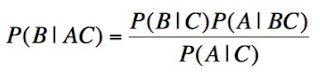
Equating the right hand sides of each of these and dividing one factor across yields Bayes' theorem in its most general form:
Above, P(B | C) is the prior probability for B, conditional upon C. A is some information additional to the prior information. P(A | BC) is the probability for A, given B and C, termed the likelihood function. P(A | C) is the probability for A, regardless whether or not B is true. Finally, P(B | AC) is the posterior probability for B, once the additional information is added to the background knowledge.
For convenience, the A in the denominator on the right hand side of this expression is often resolved into a set of relevant, mutually exclusive (meaning that the probability for more than 1 of them to be true is zero) and exhaustive (they must account for all possible ways that A could be true) 'basis' propositions. A simple example is as AB and AB' (B' denoting "B is false"). This usually allows the denominator to be split up into a sum of terms that can be more easily calculated. For example:
P(A | C) = P(AB + AB' | C)
Applying the extended sum rule (noting again the mutual exclusivity) and the product rule to each of the resulting terms gives:
P(A | C) = P(B | C)P(A | BC) + P(B' | C)P(A | BC)
If desired, we can extend this procedure to 3 'basis' propositions by further resolving AB' into 2 further non-overlapping propositions, and into 4 propositions, and so on, ad infinitum, if wished.
In a typical hypothesis testing application, the hypothesis space includes n hypotheses, (H1, H2, H3, ..., Hn). The background knowledge, consisting of the prior information and some model, is labelled I. Finally the novel information used to update the prior constitutes some set of empirical observations, known as the data, D. Substituting these into the general form, above, gives meaning to the abstract symbols, providing a more user-friendly version of Bayes' theorem:
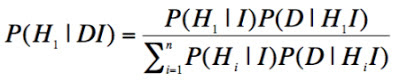
The Σ in the above formula denotes summation over the entire hypothesis space. In cases where the hypothesis space is continuous, rather than discrete, the summation becomes an integral.
Related Entries:
Related Blog Posts:
The Base Rate Fallacy was my first blog post that introduced Bayes' theorem, providing a common-sense derivation for a problem with two competing hypotheses
How To Make Ad-Hominem Arguments illustrates an instance of testing infinite hypotheses with Bayes' theorem.
External Links:
Bayes, Thomas, "An Essay Towards Solving a Problem in the Doctrine of Chance," Philosophical Transactions of the Royal Society of London 53 (0): 370–418 (1763). Available here.
Back to top
Bernoulli Urn Rule
The Bernoulli Urn rule is a basic principle of sampling theory, related to the probability for an event to occur in an experiment, when there is more than one possible outcome of the experiment corresponding to the event. An example is when rolling a die, the probability to obtain an even numbered face, Which can be achieved in 3 different ways: 2, 4, or 6.
The rule is derived from symmetry principles, as an extension of the principle of indifference, and thus takes as its starting point the condition that all possible outcomes of the experiment are equally likely. If there are R possible ways for statement A to be satisfied by an experiment, and N total possible different outcomes of the experiment, then the desired probability, P(A), is just R divided by N.
Thus, the probability to obtain an even number on rolling a die is 3/6 = 0.5.
The rule is readily justified by applying the extended sum rule to a uniform probability distribution across all possibilities.
Related Entries:
Indifference
Back to top
Binomial Distribution

The binomial distribution is an important probability distribution, specifying the probability for each possible number of outcomes of a given type, in a class of experiments known as sampling with replacement, when there are only two possible types of outcome.
Sampling with replacement means that each sample is drawn from the same population. The probabilities associated with each type of outcome are therefore constant throughout the experiment. One of these probabilities is usually labelled p. From the sum rule, the other probability is 1-p. A typical example of sampling with replacement under such conditions is repeated tossing of a coin.
We can attach arbitrary labels, '0' and '1' to the two types of possible outcome in a Bernoulli trial. Lets say the probability for a '1' is p. (Many authors label this outcome as a 'success', but we don't want to disguise the generality of the formalism.)
A given sequence of n samples, say '00110111', constitutes a conjunction of, in this example, a '0' at the first location, a '0' at the second location, a '1' at the third location, a '1' in the fourth location, etc. The prior probability to have obtained this sequence, from the product rule, is therefore (1-p)(1-p)pp.... or, since there are k '1's and n-k '0's, this probability can be expressed as pk (1-p)n-k.
From the expression just derived, it is clear that the probability with which any particular sequence of k '1's in n trials appears is independent of the order of the sequence. The proposition "k '1's in n trials", however, is a conjunction of all the possible (mutually exclusive) sequences with exactly k '1's, and so the probabilities needed for the binomial distribution are given by the extended sum rule: pk (1-p)n-k must be multiplied by the number of ways to distribute the k '1's over the n trials. The situation is analogous to randomly throwing k pebbles into n (unique) buckets (where k < n), without caring in what order the k buckets are selected. The number of distinct possibilities is the number of combinations, nCk.
The expression for the binomial distribution is therefore:
An example of a binomial probability mass function is plotted, for n = 10, p = 0.3:

Important general properties of the binomial distribution are:
- mean = np
- The peak position is given by different formulae under different circumstances
(1)
|
floor([n+1]p)
|
if (n+1)p is 0 or a noninteger
|
(2)
|
(n+1)p
|
if (n+1)p ∈{1, 2, ..., n}
|
(3)
|
n
|
if (n+1)p = n+1
|
- standard deviation = √np(1-p)
Both the Poisson and normal distributions can be derived as special cases of the binomial distribution. The binomial distribution is itself a special case of the hypergeometric distribution, in the limit where the size of the sampled population is infinite (the 'sampling with replacement' condition).
Related Entries:
Boolean Algebra
Boolean algebra is a mathematical system for investigating binary propositions. Such propositions are represented by Boolean variables, whose values are limited to either 0 or 1, corresponding, respectively, to the proposition being assumed false or true. No Boolean variable can be both 0 and 1.
In the probability theory that I discuss, all propositions about the real world are assumed to be Boolean. They are exclusively either true or false, and never anything in between.
Boolean algebra was introduced by George Boole, in 1854.
The system can be most easily understood as making use of three elementary logical operations. These operations are (other notations exist for these operations):
- negation, denoted NOT(A), for some single proposition, A
- conjunction, denoted AND(A, B), for two propositions A and B
- disjunction, denoted OR(A, B), again for two propositions
All other logical operations can be derived from these three, though they do not represent a minimal set (with cascaded NAND operations (negated ANDs), these three and all others can be formed, though some intuitive appeal is lost).
The AND and OR operations can be generalized to any number of inputs. The AND operation defines a new proposition, which is true only if all the inputs are true. The OR operation returns true if any of the inputs is true. The NOT operation converts 0 to 1 and converts 1 to 0.
Common derived logical operations include NAND (negated AND), NOR (negated OR), XOR (exclusive OR), material equivalence (negated XOR), implication, and logical equivalence.
Several laws exist for the manipulation of Boolean expressions. This list of 20 or so laws on Wikipedia gives a good summary of how logical expressions can be transformed, though axiomatization of Boolean algebra is possible with only a single law (a complicated formula not included in this list).
Using these laws, simplification of complex Boolean expressions is often possible. For example, one of the laws states that AND(A, OR(A, B)) = A, which complies with common sense. If A is true, then 'A or B' is also true, and the expression is true, while if A is false, any expression of the kind 'A and X' is false, so the expression is false.
The process of reducing a logical expression to its simplest form is known as Boolean minimization.
Arithmetic and many forms of logic needed for rationality can be performed using Boolean algebra. For example, 2 numbers expressed in binary form (base 2) can be added using arrays of full adder circuits, which are composed of elements performing the equivalent of AND, OR, and NOT operations.
In digital electronic circuits, Boolean computations are typically performed on inputs using networks of transistors. A circuit that implements a basic Boolean operation is known as a logic gate.
Related Entries:
not
conjunction
disjunction
Related Blog Posts:
The Full Adder Circuit
Back to top
Calibration
Calibration is the process of inferring the relationship between the states of a measuring instrument, and the possible states of nature that cause them.
Often, calibration is considered to consist of finding the condition of nature that is the most likely cause of each available state of the instrument. A more complete calibration process, however, involves inferring for each output state of the instrument, s, a probability distribution, P(c | s I), over the possibly true conditions, c, of reality.
Such a probability distribution encodes useful information such as the amount of uncertainty associated with a measurement (its error bar), and the presence of any systematic bias in the behaviour of a measuring device. Any non-systematic variability of an instrument is termed noise.
Calibration is performed by examining the output of the instrument for a number of standard input conditions, assumed to obey some set of symmetry relationships.
For example, the standard kilogram is a block of metal used for calibration of instruments for measuring mass. Assumed symmetries for this standard include the postulate that the mass of the standard kilogram does not vary with time (something now known to be false).
Calibration standards are usually kept under very highly controlled environmental conditions to reduce the probability for their associated symmetry conditions to be significantly violated.
Symmetries also must be inferred in relation to the behaviour of the instrument, such as the exact correctness of the law of the lever, under all circumstances, when using a weighing balance for the measurement mass.
Because of the need to assume such symmetries, whose validity can only be established using additional instrumentation, itself relying on further assumed principles of conservation, calibration of an instrument is always necessarily probabilistic. This condition is referred to here as the calibration problem. This reliance on supposed symmetry is equivalent to the problem of theory ladenness.
Related Entries:
Noise
Theory Ladenness
Related Blog Posts:
Calibrating An X-ray Spectrometer - First Steps
Calibrating An X-ray Spectrometer - Spectral Distortion
The Calibration Problem: Why Science Is Not Deductive
Back to top
Combination
A combination is a sampling of k objects from a population of n objects, for which the order of the drawn objects is undefined or irrelevant. Each ordering of any particular k objects is an instance of the same combination.
The notation for the number of possible combinations given n and k is nCk. An alternative notation consists of a pair of round brackets, containing the number n positioned directly above the number k, as shown below.
Because each combination consists of several orderings of objects, the number of possible combinations for any (n, k) is less than the number of permutations. For a sample of k objects, there are k! possible orderings, meaning that the number of possible combinations is the number of possible permutations, divided by k!:

The above expression is termed a binomial coefficient.
The counting of combinations constitutes one of two indispensable capabilities, (the other being the counting of permutations) in the calculation of sampling distributions. Sampling distributions are themselves of vital importance in the making of predictions (so called 'forward' probabilities) and in the calculation of the likelihood functions used in hypothesis testing (so called 'inverse' problems).
Related Entries:
Confidence Interval
A confidence interval (C.I.) is a region in which the true value of some estimated parameter is inferred with high confidence to reside.
Since confidence intervals relate to degrees of belief, it seems obvious that their determination should depend on the calculation of probabilities. Furthermore, since rationality demands that all relevant available information be taken into account when quantifying degrees of belief, it follows that a confidence interval should be derived from a posterior distribution.
Unfortunately, the standard definition of a confidence interval does not insist on this. Consequently, many confidence intervals do not do exactly what was expected or hoped for by their architects, sometimes to the point of delivering grossly misleading impressions.
A great deal of confusion results from the standard definition of confidence intervals, which has led me to make use of my own unconventional definition, which is guaranteed to do what every confidence interval should:
Important note:
This is not the standard definition of a confidence interval.
My definition complies with the standard definition, though, (all C.I.s obtainable using my criterion constitute a subset of all intervals compatible with the orthodox definition), while narrowing it in a way that ensures that the resulting intervals will have all the properties that a confidence interval rationally should have. For example, my C.I.s have the property that a wider confidence interval always results from a less precise measurement. This is not guaranteed under the standard nomenclature (see my blog post, and literature cited there).
In a one-dimensional parameter estimation problem, such an interval would be a line segment, (L, U), specified in terms of lower (L) and upper (U) confidence limits. Such a pair of limits specifies a convenient form of error bar.
In a two-dimensional case, the confidence interval will be the area bounded by some closed curve. For a bivariate normal distribution, for example, the confidence interval will be an ellipse.
Note that even having specified X, and having determined a posterior distribution, there are many possible confidence intervals. In 1D, for example, one can imagine obtaining a C.I. centered on the mean of the distribution, and then obtaining another C.I. by reducing both L and U by small amounts, such that the enclosed posterior density remains the same.
Normally, one is interested in the narrowest possible interval, containing some point estimate of the parameter (e.g. expectation, or median).
A confidence interval (C.I.) is a region in which the true value of some estimated parameter is inferred with high confidence to reside.
Since confidence intervals relate to degrees of belief, it seems obvious that their determination should depend on the calculation of probabilities. Furthermore, since rationality demands that all relevant available information be taken into account when quantifying degrees of belief, it follows that a confidence interval should be derived from a posterior distribution.
Unfortunately, the standard definition of a confidence interval does not insist on this. Consequently, many confidence intervals do not do exactly what was expected or hoped for by their architects, sometimes to the point of delivering grossly misleading impressions.
A great deal of confusion results from the standard definition of confidence intervals, which has led me to make use of my own unconventional definition, which is guaranteed to do what every confidence interval should:
An X% confidence interval is a connected subset of the hypothesis space that has a posterior probability of X to contain the true state of the world.
Important note:
This is not the standard definition of a confidence interval.
My definition complies with the standard definition, though, (all C.I.s obtainable using my criterion constitute a subset of all intervals compatible with the orthodox definition), while narrowing it in a way that ensures that the resulting intervals will have all the properties that a confidence interval rationally should have. For example, my C.I.s have the property that a wider confidence interval always results from a less precise measurement. This is not guaranteed under the standard nomenclature (see my blog post, and literature cited there).
In a one-dimensional parameter estimation problem, such an interval would be a line segment, (L, U), specified in terms of lower (L) and upper (U) confidence limits. Such a pair of limits specifies a convenient form of error bar.
In a two-dimensional case, the confidence interval will be the area bounded by some closed curve. For a bivariate normal distribution, for example, the confidence interval will be an ellipse.
Note that even having specified X, and having determined a posterior distribution, there are many possible confidence intervals. In 1D, for example, one can imagine obtaining a C.I. centered on the mean of the distribution, and then obtaining another C.I. by reducing both L and U by small amounts, such that the enclosed posterior density remains the same.
Normally, one is interested in the narrowest possible interval, containing some point estimate of the parameter (e.g. expectation, or median).
Related Entries:
Back to top
Conjunction
A conjunction is a logical proposition asserting that two or more sub-propositions (e.g. X and Y) are both true. Different ways of denoting such a proposition are 'XY', 'X.Y', and 'X∧Y'. These notations can be read as 'X and Y are true'. Sometimes when expressing probabilities, a comma is used to express a conjunction, as in P(X,Y), or P(Z | X,Y). The probability associated with a conjunction is obtained from the product rule, a basic theorem of probability theory.
Using a 1 to represent 'true' and a zero to represent 'false', the truth table for the conjunction of X and Y is as shown below. For each of the possible combinations of values for X and Y (left-hand and centre columns), the truth of the conjunction is shown (right-hand column). As indicated, X.Y is only true when X is true and Y is true:
| X | Y | X.Y |
| 0 | 0 |
0
|
| 0 | 1 |
0
|
| 1 | 0 |
0
|
| 1 | 1 |
1
|
Related Entries:
Back to top
Consequentialism
Consequentialism is a branch of moral philosophy, in which it is believed that only the expected results of one's actions determine whether one's actions are optimal.
This contrasts most strongly with absolutism, which asserts that there exist absolute principles of morality that hold, irrespective of the consequences of one's actions.
Consequentialism (or a subset of it, at least) can be shown to be the only correct point of view, by making use of simple statements that follow automatically from an uncontroversial understanding of the meaning of the word 'good,' as explained in the blog post, Scientific Morality. These arguments are further built upon in another post, Crime and Punishment.
The consequentialism that I defend is distinct from 'actual consequentialism,' which is the belief that only actual consequences determine whether a person's behaviour is moral. This position is indefensible, however, as it allows no way to distinguish between an action based on sound reasoning from high-quality evidence, that nonetheless fails to produce a good outcome, and an action based on willful ignorance and irrationality, that also fails. Coherence demands, however, that is is better to be wrong for good reasons, than to be equally wrong for bad reasons (my blog post, Is Rationality Desirable?, goes into far greater depth than this hand waving argument). Thus, an action is morally better than another if its outcome is expected, under reliable reasoning, to be better than the outcome of the other action.
An action with optimal results, therefore, may not be morally better than another with sub-optimal results, if, for example, prior to the event only an idiot would have predicted a good outcome.
An action with optimal results, therefore, may not be morally better than another with sub-optimal results, if, for example, prior to the event only an idiot would have predicted a good outcome.
Conventional thought finds difficulty reaching the conclusion that uniquely true assessments of value exist as matters of fact, and hence that consequences can be objectively classified as better or worse, but since value is a property of conscious experience, there can be no doubt such a thing exists, and hence that statements about value are either true or false. The quality of an assessment of value, though, obviously depends on the quality of our moral science.
Related Entries:
Related Blog Posts:
Back to top
Cumulative Distribution Function
The cumulative distribution function, or CDF, F(x), is the integral of a probability distribution function, f(x), from -∞ to x.
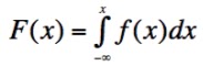
From the extended sum rule, it is clear that this corresponds to the probability that any one of the hypotheses in the region from X = -∞ to X = x is true:
F(x) = P(X ≤ x)
From the definition of the definite integral, it is clear that the probability associated with a composite hypothesis, a < x ≤ b, is given by
P(a < x ≤ b) = F(b) - F(a)
As an example of the CDF, the plot below shows the CDF (red curve) of a normal distribution (blue curve). Note that the two curves are plotted on different scales - in reality, the CDF is at all points higher then the PDF.

The complement of the CDF is termed the survival function, and the inverse of the CDF is termed the quantile function.
Related Entries:
Derivative
The derivative of a function of x, y = f(x), at some point, x0, is loosely defined as the rate of change of the function at x0. More precisely, it is the slope of the tangent line to the curve traced by f(x) at that point (assuming that f(x) is differentiable). (A tangent line is a line touching the curve at exactly one point.)
Three common notations for a derivative are dy/dx, f'(x), and y'.
Imagine two points on the curve, f(x): one at x0, and the other positioned a distance h, further down the x-axis. The slope of the line through these two points is:

As h gets smaller and smaller, we get closer to obtaining the slope of the tangent in the definition of the derivative. Mathematically, we take the limit of the above formula, as h gets arbitrarily close to, but not equal to zero:

Using this expression, certain standard derivatives have been worked out, and some of the common ones are summarized in the table below.
For example, using the results for powers of x, and for a sum of functions, the derivative of a polynomial function such as the cubic function, y = 2x3 - 2x2 - 6x + 10, can be easily worked out by formula. The graph below shows this function (blue curve). The formula for the derivative, dy/dx, is worked out from the rules in the table (items 1, 2, and 6), and is included on the graph. Choosing some value of x (x = -1, as it happens), the derivative at that location is found from the formula for dy/dx to be 4, and the corresponding y value (y = 12) is obtained from the original formula for the function. With the x-value, the y-value, and the slope of the tangent line (dy/dx), the tangent line is completely specified, and is also plotted (red line):

As long as a curve, f(x), is smoothly varying, the derivative can be found at all x positions on the curve using the above procedure, or using some numerical approximation. Numerical approximation of dy/dx consists of computing Δy/Δx for two points separated, in x coordinate, by some very small distance, Δx.
The process of calculating a derivative is termed differentiation.
The derivative is one of two fundamentally important concepts in the mathematical discipline known as calculus. The other concept is the integral. The fundamental theorem of calculus relates derivatives to integrals. Approximately speaking, taking the integral of a derivative returns the original function, and vice versa, taking the derivative of an integral returns the original function.
A turning point of a function, where the function passes through a local peak or trough, is characterized by the slope of the function changing from positive to negative, or vice versa. At the turning point, therefore the derivative is zero. Solving for the roots of f'(x) thus give the turning points of f(x).
Table of standard derivatives:
Item
|
Situation
|
y = f(x)
|
f'(x)
|
a constant |
c
|
0
| |
A sum of functions |
u(x) + v(x)
|
u'(x) + v'(x)
| |
3 | A product of functions |
u(x)v(x)
|
u(x)v'(x) + v(x)u'(x)
|
Quotient of functions |  |  | |
Chain rule
(see note below) |
y = g(u), u = h(x)
|  | |
Powers of x |
cxn
|
cnx(n-1)
| |
Exponential |
ekx
|
k ekx
| |
Number raised to the power x |
ax
|
ax ln(a)
| |
Natural logarithm |
ln(x)
|  | |
Other logarithms |
loga(x)
|  | |
Sine |
sin(x)
|
cos(x)
| |
Cosine |
cos(x)
|
-sin(x)
| |
Tangent |
tan(x)
|
sec2(x)
| |
Secant |
sec(x)
|
sec(x)tan(x)
| |
Cosecant |
cosec(x)
|
-cosec(x)cotan(x)
| |
Hyperbolic sine |
sinh(x)
|
cosh(x)
| |
Hypoerbolic cosine |
cosh(h)
|
sinh(x)
| |
Arc sine |
sin-1(x)
|  | |
Arc cosine |
cos-1(x)
|  | |
Arc tangent |
tan-1(x)
|  | |
Arc hypoerbolic sine |
sinh-1(x)
|  | |
Arc hypoerbolic cosine |
cosh-1(x)
|  | |
Arc hypoerbolic tangent |
tanh-1(x)
|  |
Of particular note in the table is item 5, the chain rule. Using the chain rule, composite functions built out of several of the above standard functions can be differentiated. For example, item 8 gives the derivative of a constant raised to the power of x. A function, g(u) = ah(x), consisting of a constant raised to the power of a function of x is differentiated by setting u equal to the exponent, h(x), and taking the product of two standard derivatives, exactly as prescribed by the above formulation of the chain rule. Higher-order nesting of functions can be attacked by applying the chain rule repeatedly.
Related Entries:
Disjunction
A disjunction is a logical proposition asserting that at least one of two or more sub-propositions is true. Up to all the sub-propositions referred to by a disjunction may be true, for the disjunction to hold (this is distinct from the logical XOR operation - exclusive or - which asserts that exactly one of the sub-propositions is true). For two propositions, X and Y, the disjunction is typically written 'X+Y', which is read 'X or Y'. Another notation is 'X∨Y'.
A disjunction is a logical proposition asserting that at least one of two or more sub-propositions is true. Up to all the sub-propositions referred to by a disjunction may be true, for the disjunction to hold (this is distinct from the logical XOR operation - exclusive or - which asserts that exactly one of the sub-propositions is true). For two propositions, X and Y, the disjunction is typically written 'X+Y', which is read 'X or Y'. Another notation is 'X∨Y'.
The extended sum rule, a basic theorem of probability theory specifies the probability for a disjunction, P(A+B).
Using a 1 to represent 'true' and a zero to represent 'false', the truth table for the disjunction, X+Y, is as shown below. For each of the possible combinations of values for X and Y (left-hand and centre columns), the truth of the disjunction is shown (right-hand column). As indicated, X+Y is only false when X is false and Y is false:
Using a 1 to represent 'true' and a zero to represent 'false', the truth table for the disjunction, X+Y, is as shown below. For each of the possible combinations of values for X and Y (left-hand and centre columns), the truth of the disjunction is shown (right-hand column). As indicated, X+Y is only false when X is false and Y is false:
| X | Y | X+Y |
| 0 | 0 |
0
|
| 0 | 1 |
1
|
| 1 | 0 |
1
|
| 1 | 1 |
1
|
Related Entries:
Conjunction
Extended sum rule
Back to top
Effect Size
Effect size is a measure of the distance between two probability distributions over similar hypothesis spaces. It is used to quantify the magnitude of an effect.
For example, if farmers found that wearing pink T-shirts made potatoes grow larger, a crude measure of effect size would be the difference between the average size of a potato grown by a pink T-shirt wearing farmer and a non pink T-shirt wearing farmer. The probability distributions in question concern the size of a randomly sampled potato, and the continuous hypothesis space is e.g. potato mass.
More usually, measures of effect size are standardized to account for the width of the effect-free probability distribution. Thus, staying with the potato example, if the mass of a randomly sampled potato, grown by a non pink T-shirt wearer, is 500 g ± 200 g, an increase to only 520 g average mass for the pink T-shirt wearer represents only a small effect size. Many of the treated cases will be smaller than many of the untreated cases, and if wearing a pink T-shirt happens to be costly, it may not be economical to apply this treatment, even though it increases yield.
The are many measures of effect size, but an unqualified use of the term usually refers to the difference between the means for the with-effect and without-effect cases, divided by the standard deviation (assuming this is the same for both cases).
Back to top
Evidence
Evidence is any empirical data that when logically analyzed results in some change to the assessment of the reliability of some hypothesis.
When measured in decibels, the evidence for a proposition, A, is given in terms of the logarithm of the odds for A, O(A):
E(A) = 10 × log10(O(A))
When the evidence is 0 dB, therefore, the proposition A is equally as likely as its compliment, A'. Evidence amounting to about 30 dB corresponds to P(A) = 0.999. Not surprisingly, a probability of 0.001 corresponds to evidence of about -30 dB (E(A) = -E(A')).
Rather than quantifying the totality of evidence for A (which demands specification of a prior), it is possible to give the amount of change of evidence supported by some set of data. This change of evidence is also termed 'evidence'. It is calculated by replacing the odds, O(A), in the above formula, by the ratio of the likelihood functions for A and its compliment, A'. Because the evidence is a logarithmic function, the posterior evidence is given simply as the sum of the prior evidence and this relative evidence associated with the data.
Some authors claim that the use of the base 10 and the factor of 10 give a general psychological advantage when it comes to appreciating and interpreting evidence quantified in dB.
Related Entries:
Odds
Likelihood Function
Back to top
Expectation
The expectation of a distribution is the centre of mass of that distribution. It is one of the most common measures of the location of a probability distribution. Other common terms for the expectation are the mean and the average.
If a probability distribution describes the likely outcomes when sampling a random variable, X, then the expectation is denoted with angled brackets, thus:
μx = 〈X〉
Under many circumstances, (corresponding to a common class of utility function)〈X〉is considered to be our best possible guess for the value of a sample from this distribution, x (i.e. an instance of the random variable, X).
For a discrete distribution, the expectation is calculated using the following formula:

The following formula is used for a continuous distribution:

The motivation for these formulas is described in another entry on the concept of mean, together with discussion of their interpretation and important distinctions between the expectation and other measures of location.
Related Entries:
mean
Related Blog Posts:
Great Expectations discusses further properties of expectations.
Back to top
The extended sum rule is a basic theorem of probability theory, specifying the probability associated with a disjunction, A+B.
The rule is derived easily from the sum and product rules, and is written:
P(A+B | C) = P(A | C) + P(B | C) - P(AB | C)
Often, for convenience, a proposition will be resolved into a disjunction of mutually exclusive 'basis' propositions, in which case the probability associated with the conjunction, AB, is zero, and the rule simplifies.
The rationale behind the extended sum rule is intuitively appreciated by drawing a Venn diagram to represent the sample space, consisting of 2 interlocking circles, one for A and the other for B (see figure). We imagine the areas of the circles to be proportional to P(A) and P(B) respectively. The region of overlap is thus proportional to P(AB). The sum, P(A) + P(B), therefore, counts the overlap P(AB) twice, so to determine P(A+B), this overlap needs to be subtracted.

By drawing the appropriate truth table, we can easily confirm that the negation of the disjunction A+B is the same proposition as A'.B', "not A and not B" (note that A'.B' and (A.B)' are not the same):
Applying the sum rule (SR) and inserting this substitution, and then also applying the product rule (PR), we can proceed to towards our goal:
From the last line, above, we simply multiply out the terms and apply the product rule one final time to arrive at the extended sum rule:
The extended sum rule is one of three basic theorems of probability theory, the other two being the product rule and the sum rule.
| A | B | A+B | A'.B' |
| 0 | 0 |
0
| 1 |
| 0 | 1 |
1
| 0 |
| 1 | 0 |
1
|
0
|
| 1 | 1 |
1
|
0
|
Applying the sum rule (SR) and inserting this substitution, and then also applying the product rule (PR), we can proceed to towards our goal:
| P(A+B | C) | = 1 - P(A'.B' | C) | .... | (SR) |
| = 1 - P(A' | C) × P(B' | A'C) |
....
| (PR) | |
| = 1 - P(A' | C) × [1 - P(B | A'C)] |
....
| (SR) | |
| = P(A | C) + P(A'.B | C) |
....
|
(SR & PR)
| |
| = P(A | C) + P(B | C) × P(A' | BC) |
....
|
(PR)
| |
| = P(A | C) + P(B | C) × [1 - P(A | BC)] |
....
|
(SR)
| |
P(A+B | C) = P(A | C) + P(B | C) - P(AB | C)
In the case of disjoint propositions, the extended sum rule is easily generalized to more than 2 propositions. Suppose we start with exclusive propositions A1 and B. Then we have:
P(A1+B | C) = P(A1 | C) + P(B | C)
Now, we recognise that B actually can arise in either of two possible ways, thus,
B = A2+ A3
Consequently, P(B | C) = P(A2 | C) + P(A3 | C), and the disjunction of these 3 events is
P(A1+A2+A3| C) = P(A1 | C) + P(A2 | C) + P(A3 | C)
This process could be extended, for example, by further resolving A3 into a durther conjunction, and so on.
Other, more general, generalizations are possible.
Related Entries:
Conjunction
Disjunction
Back to top
False Negative Rate
The false negative rate, often denoted as β, is the probability that an instrument will yield 'false' as output, given that the state of reality (with respect to the question posed to the instrument) is 'true'.
The false negative rate is closely analogous to the false positive rate, and further explanation of the concept can be found under that entry.
False negatives are also known as 'type II errors.'
The false negative rate is the frequency with which false negatives occur, relative to the total frequency with which the state of reality is 'true'. Thus, stated as a formula, the false negative rate is:

Since the sensitivity of a test is the probability that the instrument will infer 'true,' given that the state of reality is 'true,' another formula for the false positive rate is:

Related Entries:
False Positive Rate
Sensitivity
Specificity
Back to top
False Positive Rate
The false positive rate, often denoted as α, is the probability that an instrument will yield 'true' as output, given that the state of reality (with respect to the question posed to the instrument) is 'false'.
Sometimes, an instrument must provide an output that is binary: does the subject have the disease or not? Should the fire alarm be activated or not? Was that small region of the hard drive encoded with a 0 or a 1? Etc.
The output of the instrument must be either positive or negative. On the other hand, the state of reality, with respect to the current question, must be either 'true' or 'false'. These two categories are not always the same (one refers to the state of the instrument, and the other refers to the system that the instrument is trying to diagnose).
A false positive, therefore, is an instance where the instrument outputs 'positive,' i.e. infers reality's state to be 'true,' even though reality's state is actually 'false.' False positives are also termed 'type I errors.' We need to be careful with the terminology, however - the 'false' in 'false positive,' refers not to the state of reality, but to the correctness of the instrument's diagnosis. Thus, a true negative is a case where the instrument infers reality's state to be 'false', and this inference is correct.
The false positive rate is, therefore, the frequency with which false positives occur, relative to the total frequency with which the state of reality is 'false'. Thus, stated as a formula, the false positive rate is:

Since the specificity of a test is the probability that the instrument will infer 'false,' given that the state of reality is 'false,' another formula for the false positive rate is:

In general, designing an instrument involves choosing an appropriate trade-off between false positive rate and false negative rate, as decreasing one is most easy to do by increasing the other.
Related Entries:
False Negative Rate
Sensitivity
Specificity
Back to top
Falsifiability Principle
The falsifiability principle asserts that in order for a proposition to be scientific, and suitable for scientific investigation, it must be vulnerable to falsification.
The principle was originated by Karl Popper, and is more commonly known as the falsification principle. At Maximum Entropy, however, the term falsifiability is preferred as it seems more precise, the traditional term being often misinterpreted, by scientists and 'lay people' alike, to imply that the purpose of science is to falsify theories. Correctly interpreted, falsifiability is to be seen as a demarcation criterion, dividing propositions into those that are useful and those that aren't.
Relatedly, Popper believed that falsification was the only way for knowledge to advance, but this is incompatible with a rational view point, as, in light of new information, probabilities may be altered upwards or downwards, and in increments almost always less than those required to reach maximal certainty.
The falsifiability criterion can be understood in terms of the likelihood function associated with some data set, D. If a theory, H, is unfalsifiable then the likelihood, P(D | HI), will always be high (relative to the peak of the likelihood), regardless what data have been observed. No useful predictions are possible with such a theory. Assigning a high probability to H, therefore, teaches us nothing about nature, and the theory is useless. The term 'pseudoscience' is often used for such theories.
Unfalsifiable theories also necessarily possess infinite degrees of freedom (an unlimited number of fitting parameters), which I argue necessarily assigns to them strictly zero prior probability. Unfalsifiable theories are not, therefore, untestable, as many assume. One only needs to postulate the existence of an alternate hypothesis with finite degrees of freedom (which is always a sound premise) in order to automatically assign a probability of zero to such theories, making them the most readily testable propositions going around.
Related Entries:
Related Blog Posts:
Bayes' Theorem: All You Need to Know About Theology describes the impact of the infinite degrees of freedom of unfalsifiable theories
Inductive inference or deductive falsification? shows that falsification is just another bog-standard part of inductive inference
Back to top
Frequency Interpretation
The frequency interpretation of probability is a popular but severely flawed understanding of the meaning of probabilities. According to the frequency interpretation, each probability corresponds to a physical frequency. This means that the probability associated with some event is the same as the relative frequency with which that event will occur in some infinite set of physical experiments.
For example, in a coin tossing experiment the relative frequency with which the coin lands with the head facing up might be 0.5, which, typically would also be the probability, P(head). In this case, the frequency and the probability are the same.
The correspondence breaks down, however, in several trivial ways. In the coin tossing example, before any trials have been performed, and with no pertinent information to the contrary, symmetry demands that I assign 50% probability to the occurrence of a head. The physical coin, however, along with the tossing procedure, may be biased to produce some different frequency of outcomes, and so the probability is more properly seen not as a physical frequency, but as a statement of one's available knowledge about the experiment.
The frequency interpretation breaks down even more dramatically when considering the probability for propositions such as "the universe is between 13.7 and 13.9 billion years old." There is no sense in which the truth of such statements can vary with any frequency.
Some have tried to rescue the frequency interpretation by arguing that among the set of all hypotheses for which the probability is x, the fraction that are true is x, and that x is therefore a physical frequency. This, however, makes some important errors.
Firstly, every probability is determined, assuming the truth of some model, and can not be divorced from that model. It is trivial for me to test the same hypothesis within two separate models, arriving at two different probabilities. The proposed, rescued frequency interpretation, however, is powerless to say which probability is the correct physical frequency.
Secondly, given what we know about the procedures used to generate hypotheses, it is surely the normal thing for our theories to be false, no matter what probability they attain. For a long time, for example, it appeared that the universe obeyed Newtonian mechanics. Physics was then a matter of solving certain equations, with the numerical results of this procedure evidently attaining high probability. We now know (with high confidence) that reality is not Newtonian, and that all these results were, in fact, false. As false, in fact, as the results of stone-age divination techniques, though not equally wrong, of course. The falsification of Newtonian physics was a normal part of science, and there is no valid reason to expect this kind of thing to stop any time soon. A probability, therefore, is no more than an expected frequency, assuming the truth of some model. It is, consequently, not a physical parameter, but an imagined entity.
Adherents of the frequency interpretation are known as frequentists.
Traditional favourite techniques of frequentists most notably include null-hypothesis significance testing and maximum likelihood parameter estimation, though each of these, sadly, commits the base-rate fallacy, resulting in limited validity.
Traditional favourite techniques of frequentists most notably include null-hypothesis significance testing and maximum likelihood parameter estimation, though each of these, sadly, commits the base-rate fallacy, resulting in limited validity.
Related Entries:
Related Blog Posts:
The Mind Projection Fallacy
Parameter Estimation and the Relativity of Wrong
Insignificance of Significance Tests (discusses the flaws inherent in null-hypothesis significance testing)
Fly Papers and Photon Detectors (illustrates the breakdown of maximum-likelihood parameter estimation)
Parameter Estimation and the Relativity of Wrong
Insignificance of Significance Tests (discusses the flaws inherent in null-hypothesis significance testing)
Fly Papers and Photon Detectors (illustrates the breakdown of maximum-likelihood parameter estimation)
Gaussian Distribution

Another name for the normal distribution.
Related Entries:
Hypothesis Test
A hypothesis test is a procedure for ranking the reliability of propositions about the real world by performing computations on some data set.
This is a more general definition than some specialists use, as some reserve the phrase 'hypothesis test' to refer to null-hypothesis significance tests. On Maximum Entropy, however, NHSTs are considered a special case, just one of many special-case classes of procedures, whose ultimate purpose is to mimic with varying success the output of Bayes' Theorem.
Null-hypothesis significance tests examine only a single hypothesis (the null hypothesis), and provide binary output (rejection of or failure to reject the null hypothesis).
Hypothesis tests based directly on Bayes' theorem offer a continuous range of outputs, from 0 to 1, constituting a posterior probability assignment. They can assess any integer number of hypotheses from 2 (binary hypothesis tests) up, and using differential calculus, can be applied to problems with infinite numbers of hypotheses.
Important classes of Bayesian hypothesis test are parameter estimation and model comparison.
Related Entries:
Bayes' Theorem
null-hypothesis significance tests
parameter estimation
model comparison
posterior probability
null-hypothesis significance tests
parameter estimation
model comparison
posterior probability
Related Blog Posts:
The Base Rate Fallacy introduces binary hypothesis testing
How To Make Ad Hominem Arguments introduces infinite hypothesis testing
Parameter Estimation and the Relativity of Wrong concerns parameter estimation
Ockham's Razor discusses model comparison
How To Make Ad Hominem Arguments introduces infinite hypothesis testing
Parameter Estimation and the Relativity of Wrong concerns parameter estimation
Ockham's Razor discusses model comparison
Indifference
Indifference is one of a class of symmetry principles used to specify prior probability distributions.
Such principles derive from the basic desideratum that equivalent states of information lead to the same probability assignment.
The principle of indifference can be applied to all discrete distributions, under the circumstances of 'complete ignorance.' Complete ignorance implies that there is insufficient reason to favor one hypothesis over any other, and so symmetry demands that each hypothesis is assigned equal probability. Thus, when there are n hypotheses, the prior distribution from indifference is uniform, and from the normalization requirement, is equal to 1/n, for all hypotheses.
Under strict Bayesian reasoning, complete ignorance holds for the first iteration of Bayes' theorem. We might be told by a trusted source, for example, that a particular non-uniform prior is appropriate. In such a case, however, before the problem can be evaluated, rationality demands a necessary pre-evaluation of the probability that the source of the information is trustworthy. Such calculations are most often performed approximately and subconsciously.
Not all continuous distributions can be analyzed by the principle of indifference for the condition of maximal ignorance. This is because the resulting distribution is not generally invariant under transformations of the parameter space.
For example, if we are told that a square has sides of length between 5 and 10 cm, we might consider all lengths in this range to be equally probable. The given prior information, however, is equivalent to the statement that the area of the square is between 25 and 100 cm2, suggesting just as much that all areas in this range are equally likely. The second distribution, unfortunately, is not equivalent to the first. Since there is no compelling reason to give precedence to either the length or the area, some other method, such as the principle of transformation groups, must be used instead to determine the appropriate ignorance prior.
The principle of indifference can also be derived from the principle of maximum entropy, as shown in this blog post.
Related Entries:
Principle of Transformation Groups
Related Blog Posts:
Integral
The indefinite integral,
∫ F(x) dx
gives the area bounded by the function, F(x), and the x-axis. The process of calculating an integral is termed integration. The function F(x) is termed the integrand.
The integral is one of two fundamentally important concepts in the mathematical discipline known as calculus. The other concept is the derivative. The fundamental theorem of calculus relates derivatives to integrals. Approximately speaking, taking the integral of a derivative returns the original function, and vice versa, taking the derivative of an integral returns the original function.
Setting the above integral, therefore equal to a function, f(x), then F(x) = f '(x) satisfies the equation. Substituting the function f(x) + c for f(x), however, also satisfies this condition, as the derivative of a constant is zero. Thus, the general solution of the above integral is some function of x, plus some unknown constant:
∫ F(x) dx = f(x) + c
In some problems, the constant of integration, c, can be determined from boundary conditions.
A selection of common integrals, obtained from first principles, are provided in the table below.
The definite integral,

gives the area bounded by the curve, F(x), the x-axis, and the lower and upper limits, a and b, respectively. When the indefinite integral is given as f(x) + c, the above definite integral is therefore given as

For example, the figure below illustrates the definite integral between limits a = -1 and b = 2 for the cubic polynomial, y = 2x3 - 2x2 - 6x + 10. The integral corresponds to the shaded area:

From the table (items 1, 3, and 4), the indefinite integral for such a polynomial can be easily obtained by formula, and is

(Note that we can apply rules 1, 2, and 6 from the table of derivatives to the above result and quickly verify that the function, y = 2x3 - 2x2 - 6x + 10 is the result.) For the limits specified, the definite integral illustrated comes to exactly 22.5.
Not all functions, F(x), have an integral that can be expressed exactly. In such cases, the integral may still be evaluated approximately, using numerical techniques. The simplest form of numerical integration is to divide the area required into a series of narrow rectangles, whose individual areas are trivial to calculate. The width of each rectangle is some small increment, Δx, and the height is given by evaluating F(x) at the centre of the interval, at x + Δx/2. The process is illustrated using the same cubic polynomial:

With only 12 intervals, the total sum over all rectangles comes to 22.48, differing from the exact result by less than 0.1%.
Table of Standard Integrals:
In the following, the solution to ∫ F(x) dx is of the form f(x) + c. The constant of integration is omitted from the table.
Item
|
Situation
|
Integrand, F(x)
|
Integral,
f(x)
|
Sum of functions
|
g(x) + h(x)
|  | |
A constant multiplying a function
|
a g(x)
|  | |
A constant
|
a
|
a x
| |
x raised to some power
|
xn
|  | |
1 divided by x
|  |
ln(|x|)
| |
Exponential function
|
ex
|
ex
| |
A constant raised to the power x
|
ax
|  | |
Sine function
|
sin(x)
|
-cos(x)
| |
Cosine function
|
cos(x)
|
sin(x)
| |
Tangent
|
tan(x)
|
-ln(cos(x))
| |
Arc sine
|
sin-1(x)
|  | |
Arc cosine
|
cos-1(x)
|  | |
Arc tangent
|
tan-1(x)
|  | |
Reciprocal root of a quadratic, 1
|  |  | |
Reciprocal root of a quadratic, 2
|  |  | |
Reciprocal quadratic, 1
|  |  | |
Reciprocal quadratic, 2
|  |  |
Many more standard integrals exist, see for example.
Techniques also exist for composite functions, such as integration by substitution (less technical introduction here), which is analogous to the chain rule for derivatives, for some functions of functions, and integration by parts for some products of functions.
Related Entries:
A joint probability is the probability associated with a conjunction. It is the probability that two or more propositions are true at the same time. A joint probability distribution gives a multi-dimensional probability density over several variables. For example, if we are interested in the current temperatures in London and New York, our relevant information could be expressed as a two-dimensional joint probability distribution, with each point in the 2D hypothesis space corresponding to a particular combination of temperatures: TL = X and TNY = Y.
An important example of a joint probability distribution is the multi-variate normal distribution.
Likelihood Function
The likelihood function gives the probability to have observed some data set, conditional upon some hypothesis, and a collection of background information, I. It is a function of the hypothesis, H, and not the data, D:
L(H) = P(D | HI)
When P(D | HI) is examined as a function of D, it is termed the sampling distribution, but it must be remembered that this is a different function, over a different domain. In particular, it is worth noting that because the likelihood function varies over the conditioning assumption, H, it is not a probability distribution function, and therefore is not normalized.
Often, the hypotheses of concern relate to the numerical values of some model parameters, θ = (θ1, θ2, θ3,...), and it's not uncommon to see the likelihood function denoted as L(θ).
The likelihood function plays an important role in Bayesian inference, and in maximum-likelihood parameter estimation.
The base-rate fallacy is a common mistake whereby inferences are drawn by looking only at the likelihood function (or something closely related), and not including the prior probability, as Bayes' theorem specifies. Under circumstances where the prior distribution is close to uniform, however, this kind of approximate reasoning may be sufficiently accurate.
Related Entries:
Marginal Distribution
A marginal distribution is a probability distribution over a parameter space of reduced dimensions. For example, if a parameter space ranges over x and y, the corresponding probability distribution is P(x, y | I). We may, however, only be interested in the probabilities associated with the various values for one of the parameters, x. The distribution of interest, P(x | I), is said to be marginalized over y. The parameter, y, is often termed a nuisance parameter.
The marginal distribution for x is given by:
The marginal distribution for x is given by:

The method required to calculate a marginal distribution arises fairly simply from the basic rules of probability. Suppose that we divide the entire parameter space over y into two non-overlapping regions, y1 and yA. Since these are the only possibilities in y-space, then the proposition, 'x' (our shorthand for 'X = x', where x is an event, and X is the random process generating that event) is logically the same as the proposition 'x and y1 or yA'. In symbols:
x ≡ x.[y1 + yA]
The probabilities for these must therefore be the same:
P(x | I) = P(x.[y1 + yA] | I)
= P(x.y1 + x.yA | I)
Employing the extended sum rule, and the fact that y1 and yA are disjoint (exclusive),
P(x | I) = P(x.y1 | I) + P(x.yA | I)
Next the product rule is invoked, yielding
P(x | I) = P(x | y1.I)P(y1| I) + P(x.yA | I)
If, however, we feel that two points is not sufficient to resolve all the possibilities in y-space, we can further resolve yA into two further propositions: y2 and yB. Thus, the last term in the above sum becomes
P(x.yA | I) = P(x.[y2 + yB] | I)
which can again be split up into a sum of 2 terms, exactly as was just done. This process can go on indefinitely, yielding a string of terms, one for each of the propositions, y1, y2, y3, y4, ... , yielding a final marginalized distribution,

In the most general case the parameter space over y will be continuous, and we can better represent the marginal distribution as an integral, where P(x) now represents a probability density:
Because P(.) is now being used to represent a probability density, with units inverse to those of the parameter space, the product P(y | I)×dy is dimensionless, and P(x | I) has the same units as P(x | y, I).
The process of marginalization can be extended to any number of dimensions. So for a distribution on three axes, P(x,y,z | I), the marginal distribution over z would be:

from which it can be seen that the marginal distribution over y and z (the distribution for x, irrespective of what y and z might be) is:

This last formula can be simplified, if y and z are conditionally independent, i.e. if P(y | z, I) = P(y | I).
Related Entries:
Nuisance Parameter
Related Blog Posts:
Maximum Entropy Principle
The maximum entropy principle is a mathematical prescription for assigning probability distributions. It is a way of figuring out an appropriate probability distribution, capturing the information one has on the problem in hand, without assuming any additional information, (beyond the necessary model assumptions), that is not possessed.
Of all the possible distributions consistent with the constraints of a given problem, the one for which the information-theoretic entropy is maximum is the one that is maximally non-committal. It entails no stronger belief than that which is inherently justified by the structure of the problem. This distribution assumes no additional information, beyond what is already known and encoded in the problem constraints, and thus provides the optimal description of the corresponding state of knowledge.
The maximum entropy principle is often used to assign prior probability distributions, before the subsequent use of Bayes' theorem to analyze the effect of some data set. It is perhaps most easily thought of as a means of providing uninformative priors. It is also possible, however, to use it for the direct assignment of posterior distributions. (The distinction between prior and posterior is arbitrary, so the theory would be inconsistent if this were not so.)
The information-theoretic entropy (also known as the Shannon entropy), denoted H, is given by the formula:
H = -Σi pi × log(pi)
where pi is the probability associated with the ith hypothesis in some discrete hypothesis space. The maximum entropy principle states that the distribution that maximizes this function is the one consistent with rationality.
A version of the above formula exists for continuous distributions.
Given a finite set of discrete hypotheses, and no further information, the maximum-entropy distribution is uniform over the hypothesis space.
For a continuous distribution with known mean and standard deviation, and no further information, entropy is maximized with the normal distribution.
Related Entries:
Related Blog Posts:
Entropy of Kangaroos introduces a very simple application example.
Entropy Games discusses the meaning of entropy.
Monkeys and Multiplicity provides an intuitive argument for the correctness of the principle.
The Acid Test of Indifference derives the uniform prior from MEP.
Maximum Likelihood
Maximum likelihood is an approximate method of parameter estimation, which involves finding the peak of the likelihood function, P(D | HI).
The method is closely associated with the frequentist tradition. It does not comply with Bayes' theorem, and it therefore does not make maximal use of available information. Its validity is limited to cases where the prior distribution is uniform, or negligibly informative, relative to the data.
Conventionally, when hypothesis testing is cast in the language of parameter estimation, the hypothesis, H, is denoted as a set of model parameters, θ = (θ1, θ2, ...), and the likelihood function is written:

The maximum-likelihood estimate of θ is often denoted with a circumflex:

The argmax() function gives the argument of L(θ), θ, at which L(θ) is maximized. Note, it is not the value of L(θ) at its maximum.
When the functional form of L(θ) is known, argmax() is often found by setting the derivative of L(θ) equal to zero and solving.
When the data set, D, consists of several individual data points, D = (d1, d2, ...), and when a normally distributed noise model is used, maximizing L(θ) amounts to minimizing the χ2 statistic (as shown in the entry on parameter estimation):

Here y(x) represents the noise PDF. If the standard deviation of the noise distribution can be treated as constant over all data points, this reduces even further, to the method of least squares, in which the sum of the squared residuals, S, is minimized:

Analytical solutions to the least-squares method exist in some cases. For example, a polynomial model of arbitrary degree can be easily solved, as shown here. For optimization of either test statistic, S or χ2, in more complex situations, numerical solvers such as the Gauss-Newton method or the related Levenberg-Marquardt algorithm can be used.
Related Entries:
Related Blog Posts:
External Links:
Mean
Most generally, the arithmetic mean of a list of numbers is the average: the sum of all the numbers divided by the count of the numbers. It can thus be seen to characterize a global property of the list.
Applied to a probability distribution, the list of numbers in question corresponds to the complete set of hypotheses in the relevant hypothesis space. However, we must consider that each element of the hypothesis space appears in the list more than once, the number of appearances of each being proportional to the probability assigned to it. Thus the mean of a probability distribution is sometimes referred to as a weighted average.
The mean of a probability distribution, often denoted by the greek letter μ (mu), is also known as the expectation, denoted by angle brackets:
μx = 〈X〉
From the weighted-average argument, we can see that for a discrete distribution, the mean is calculated using the formula:
Here, the Σ (upper-case sigma) denotes summation over the entire hypothesis space. This is actually a special case, as a discrete probability distribution can be defined on a continuous space, with the probability distribution function consisting of weighted delta functions. Thus, the more general formula for the mean (over a continuous space) is given by converting the discrete summation to an integral:
The mean of a distribution provides one measure of its location. Another measure of location is the median. The distinction between mean and median is laid out below. Another measure of location is the point of maximum probability, termed the peak, or mode. The peak and the mean often do not coincide. Many distributions do not even not possess a unique peak. The choice between different measures of location depends on how one measures cost: if it is most profitable to minimize the expected square of the difference between a parameter's estimate and its true value, then the mean is the optimal choice.
A probability distribution is often described metaphorically as consisting of mass. Within this metaphor, the mean is seen to correspond to the centre of mass: if the shape of the distribution were to be realized in some material of uniform density, such as a block of wood, then the point at which the object could be made to balance is the mean. At each point in the hypothesis space, from the law of the lever, the important number is the product of the distance of that point from the balance point and the amount of probability (mass) assigned to that point. The mean is thus the location at which the sum of all these products is zero (distances to the right are positive and to the left are negative), hence the wooden model can be made to balance at that point.
While the mean is considered as corresponding to the centre of mass, the median is the midpoint of a distribution: it is the point at which the total amount of probability to the left equals the amount to the right. For the mean, recall that the corresponding sum is weighted by distance, indicating how the mean and median are distinct.
As indicated, the terms mean and average are often used interchangeably, but there is a slight danger here. The mean of a probability distribution is a property of our available information on some set of propositions. The term average, however, suggests the result of a some real experiment, though this latter strictly corresponds to a frequency distribution, which is typically not the same as a probability distribution. See entry on the frequency interpretation of probability for more detail.
The mean of a distribution over x is also the x coordinate of the centroid of its graph, so the term centroid is sometimes used as a synonym for the mean.
Related Entries:
Median
The median of a probability distribution is a measure of the probability distribution's location. Other such measures include the mean and mode - generally these all refer to different locations in the hypothesis space, but under special circumstances they can coincide.
The median, m, is the midpoint of a distribution, the point at which the total amount of probability to the left equals the amount of probability to the right. It is therefore specified by setting the integrals up to (down to) m, from the left (right) equal:

The assignment of one half follows from the definition above, and the normalization condition for probability distributions.
The median is distinct from the mean, in the same way that the midpoint is distinct from the centre of mass. The midpoint only cares about the amount of mass on either side, and is not influenced by the relative locations of the constituent masses. The centre of mass, however, is determined not from summing constituent masses, but rather by summing the products of those masses with their distances from some point in space. (This follows from the law of the lever.)
Related Entries:
Meta-analysis
Meta-analysis is a form of systematic review, aimed at pooling data from a number of different studies, often performed by different researchers, in order to assess the totality of evidence available on some particular research question.
Studies for inclusion in a meta-analysis are usually drawn from the peer-reviewed literature. A good-quality meta-analysis will aim to include all such studies, and so will involve collecting all search results, for some appropriate set of keywords, using one or more major research databases.
Studies to be included will often be ranked for methodological quality. For example, among randomized controlled trials, study reports not including specific details of the randomization protocol may be ranked lower than those supplying the appropriate information. This is because nondisclosure of method has been found to correlate with use of inferior protocols. Once ranked, studies can be weighted, such that the amount that a study contributes to the final analysis will scale with its assessed level of reliability. In practice, it is quite often the case that studies not passing some minimal level of methodological rigor will simply be not included in the statistical analysis.
Under the highest quality meta-analysis standards, the process of ranking the reliability of each study should be performed in a way that is blinded to studies' outcomes, and other factors. This avoids the possibility of researcher bias on the part of the meta-analyst.
Once the studies have been collected and assessed for methodological rigor, the statistical results of the relevant studies are aggregated to condense the totality of evidence to a single result. Great care needs to be applied at this stage, as different studies will very often employ somewhat different research designs: naive aggregation of statistics from disparate studies can lead to spurious effects, such as Simpson's paradox.
Meta-analysis can often reveal anomalies in the research literature, such as publication bias. Using techniques such as funnel plots, meta-analysts can determine whether or not there is excess significance in the reported results. For example, if noisy data, leading to small effect sizes, consistently produce highly significant results in the literature, this will show up as an anomaly. Even though the effect may be perfectly real, the noise in the data will suggest that at least some of the data should support the non-existence of the effect. This can occur under a number of different circumstances, e.g. researchers are consistently not publishing non-significant results, studies are subject to some inadvertent bias, or researchers are committing deliberate fraud.
In medical science, one of the most active and trusted producers of meta-analyses is the Cochrane Collaboration. Many other disciplines lack a robust tradition of rigorous systematic review.
External Links:
Back to top
Mind Projection Fallacy
The mind projection fallacy is a method of flawed reasoning that assumes that aspects of one's model of reality necessarily correspond to aspects of reality.
It occurs frequently in people's reasoning about probabilities, and seems to have been instrumental in the widespread acceptance of the frequentist school of statistics during the first half of the 20th century. Under this mode of reasoning, for example, many scholars believed that a probability must necessarily correspond to a physical frequency.
Thus, for example, that statement that the probability to obtain a head when a coin is tossed is 0.5 was seen as entirely due to the fact that in a long run of coin-tossing experiments, the relative frequency of heads would be 0.5. The most immediate problem with this conclusion, however, is that under different states of information, different agents must assign different probabilities. If I have seen the tossed coin, and you have not, therefore, I will assign a probability of 1 to heads, if heads is showing, while you are still stuck with the 0.5 assignment. It is not possible, therefore, for all appropriate probability assignments to correspond to physical frequencies.
Discussions of the broad concept of random variables are also often prone to flawed reasoning in the same category.
Mind projection fallacy occurs in many other areas of thought. In physics, it has cropped up most notably, perhaps, in many descriptions of statistical mechanics (see for example brief discussion near the end of this article, and clarification in the comments of the same post) and quantum mechanics, possibly slowing down progress in these areas.
Several schools of philosophical thought, such as Platonic idealism and many strains of post-modernism, also commit this fallacy.
A great deal of technical and philosophical error can be eliminated through careful appreciation of the mind projection fallacy. Those three simple words (coined as a single phrase by Edwin Jaynes) convey an insight that is applicable in an astonishing number of situations.
Related Entries:
Related Blog Posts:
Model Comparison
Model comparison is an important class of hypothesis testing, in which probability theory is employed to rank the relative merits of different theories attempting to explain observed physical phenomena. Often, model comparison is considered to constitute hypothesis testing at a higher level than parameter estimation. While parameter estimation is concerned with evaluating the likely values of numerical constants within a particular model, model comparison is considered to relate to evaluating several different models against one another. Model comparison is therefore not concerned directly with the specific values of the parameters associated with the models under scrutiny - these values are treated as nuisance parameters.
In simple parameter estimation, we have a list of model parameters, θ, a data set, D, a model M, and general information, I. Plugged into Bayes' theorem, this results in

When we have a number of alternative models, denoted by different subscripts, the problem of assessing the probability that the jth model is the right one is just an equivalent one to that of parameter estimation, but carried out at a higher level:

The likelihood function here makes no assumption about the set of fitting parameters used, and so it decomposes into an integral over the entire parameter space (extended sum rule, with P(HiHj) = 0, for all i ≠ j):
|

and the denominator of Bayes' theorem is as usual just the summation over all n competing models, and so we get

If, for any particular model, θ = (θ1, θ2, ...) contains a large number of parameters, then the integral in the numerator of Bayes' theorem, directly above, is over a large number of dimensions, and so the normalization condition ensures that the amount of probability concentrated at any particular point will not be large. In particular, the probability mass situated at or near the maximum likelihood point will be small. Thus models with many free parameters suffer a penalty known as the Ockham factor, which ensures that they tend to have a low prior probability, compared to models with fewer parameters.
This penalty is seen as the rational justification for the heuristic principle, Ockham's razor, attributed to William of Ockham, circa 1300.
Related Entries:
Nuisance Parameters
Related Blog Posts:
The following, in the presented order, constitute a mini-sequence on model comparison:
Morality
Morality deals with the selection and execution of appropriate choices of action.
Morality, in that it concerns moral behaviour, needs to be distinguished from moral truth. Moral truths exist as facts of nature. This means that in a particular situation there is an optimum behaviour (not necessarily unique), in the sense that it produces an outcome of not lower value than any other possible behaviour. Traditionally, the existence of moral truths has been doubted, owing to the belief that the assignment of value is arbitrary, but in reality, value is demonstrably and obviously a product of the architecture of minds, and therefore exists.
As non-omniscient beings, however, we can never have perfect knowledge of the value-related consequences of each possible action we might take, and so choosing moral behaviour becomes a decision-theoretic procedure, with a crucially important grounding in probability theory. We have to do the best we can with the imprecise knowledge we have and our limited computational resources available. Behaviour can be said to be moral, therefore, even if decisions are made that work against moral truths, as long as a rational attempt has been made to assess what actions are optimal.
Thus defined, morality is heavily entwined with science. Every scientific question is a hypothetical moral question: what is an appropriate behaviour to cost-effectively maximize my knowledge of X? (Knowledge of X is not necessarily desirable, and thus scientific research may be immoral.) Every moral question is a scientific question: based on state of the art knowledge and inference techniques, what is my best estimate of the relevant moral truth? (To desire something is to desire means to maximize one's expectation to attain it, thus when assessing what behaviour is appropriate it is necessarily appropriate to utilize scientific method.)
Thus, as with literally all fields of knowledge, the state of the art in morality is only attained through application of scientific method.
Related Entries:
utility
Related Blog Posts:
The Moral Science Page provides an index of and guide to all my blog posts and glossary entries on this topic.
Scientific Morality derives the principle that moral truths exist from two analytical statements, (1) 'good' and 'evil' have no existence outside minds, and (2) morality is doing what is good.
Crime and Punishment demonstrates that the only coherent morality is consequentialism, and applies this insight to the problem of criminals.
Practical Morality, Part 1 and Practical Morality, Part 2 argue that the possibility of a moral science has important implications going far beyond mere theoretical or academic interest. The first part discusses how moral science can be attained (and in practice, actually is), while the second part outlines two areas where simply recognizing the possibility of learning moral truth though empirical investigation might have far reaching implications for society.
External Links:
Richard Carrier has developed in detail a sophisticated moral philosophy with no detectable major departures from my own moral philosophy. See for example, his Moral Ontology.
Noise
In scientific terminology, noise is that part of a set of measured data that does not improve inferences about the topic of interest, and can not be removed or reduced by improved calibration of the instrument.
In a measurement, noise contributes to uncertainty as to the true condition of the entity being measured.
Noise is the sum of all components of a measurement that, in a subjective sense, vary non-systematically. Noise, therefore, can not be removed by subtracting a constant offset, or by developing any other deterministic functional relationship between the phenomenon being measured and the output of the instrument. Such steps are part of the calibration process.
The effect of noise is that repeated measurements of the same object will produce slightly different results. Sources of noise include the limited sensitivity of the instrument, such as uncertainty when measuring very short lengths with a ruler, and intrinsic variability of the thing being measured, such as random fluctuations in the density of traffic on a road.
A more sensitive instrument, capable of distinguishing smaller changes in the quantity of interest will lead to reduced noise.
An increased number of measurements can also reduce the impact of noise. This is because the mean of a distribution is not the same as the distribution for the mean. Measurement of a quantity will have some probability distribution, determined in part by some frequency distribution for the magnitude of the noise signal, but the mean of that probability distribution can be inferred to arbitrary precision, by taking many samples.
Other methods for handling noise, such as lock-in amplification, result in a loss of information, which may be undesirable if an efficient data-analysis algorithm is to be used.
The non-noisy part of a measurement is usually termed 'signal.' The quality of a measurement is therefore often quantified in terms of the signal-to-noise ratio, or SNR. A higher SNR implies lower relative uncertainty. For a Poisson-distributed data-generating process (such as absorption in a detector of photons emitted by a candle), the signal-to-noise ratio is the square root of the signal intensity. Thus, a larger or more efficient detector often improves the SNR.
Related Blog Posts:
Signal and Noise gives an example of quantifying the impact of noise on an inference task.
Normal Distribution

The factor in front of the exponential function serves the purpose of normalization.
The normal distribution is of central importance in applied statistics, for two main reasons:
- Firstly, it is an accurate model of the frequencies associated with many physical phenomena. This is explained by the central limit theorem, which shows that adding together a large number of random processes results in a distribution that in the infinite limit is the normal distribution.
- Secondly, it is the maximum-entropy distribution, when nothing is known but the distribution's mean and standard deviation. This means that in situations where an uninformative prior is required, the normal distribution can often capture the information that we have, without forcing us to assume (potentially false) information that we don't have.
The integral of the normal distribution is given in terms of the so-called error function, erf(z). For example, the cumulative distribution function for the normal distribution is:

Several numerical approximations for the error function exist. Some programming languages and most mathematical software packages include routines to evaluate error functions. The formula for the error function is:

A simple and efficient technique for generating normally distributed random numbers from a generator of uniformly distributed random numbers is the Box-Muller method.
The standard normal distribution is a normal distribution with μ = 0 and σ = 1. Any normal distribution can be standardized by transforming the hypothesis space from x to x', where x' is (not a derivative) given by:

A plot of a normal distribution, with parameters μ = 10 and σ = 5, is plotted below (blue curve), together with its cumulative distribution function (red curve). Note that the two curves are plotted on different scales - in reality, the CDF is at all points higher then the PDF.
Related Entries:
External Links:
There's so much to know about the normal distribution that this extensive Wikipedia article is worth looking over.
Normalization Condition
The normalization condition is the requirement that the total amount of probability 'mass' over a hypothesis space adds up to 1. It follows as a direct result of the sum rule, a basic theorem of probability theory. For a discrete distribution, the amount of 'mass' is the sum of the probabilities for each of the discrete propositions in the hypothesis space. For a continuous distribution, the 'mass' is the integral over all space,

Once the shape of a probability distribution (characterized by the mean, the standard deviation, and higher moments) has been determined, normalization is ensured by dividing by the above factor.
Not all mathematical functions can be normalized. A distribution, such as the continuous uniform distribution from 0 to ∞, that can't be normalized is termed 'improper'. To smooth the computation process, an improper distribution may sometimes be replaced by a related distribution that is proper, without impacting too drastically on the results. For example, the infinitely wide uniform distribution, may be replaced with a truncated rectangular distribution. Often this process will correspond to approximately implementing existing prior information that is difficult to formally specify otherwise. One must remain mindful, of course, that not all logical consequences of an arbitrary prior will correspond exactly to a fully rational result. As with all types of arbitrary prior, sensitivity analysis can be performed by adjusting the prior and looking for variability of the results - if the arbitrary form has been appropriately chosen, then the results should not vary significantly.
Related Entries:
Not
The not operation, NOT(A), is an elementary operation in Boolean algebra (binary logic), which finds the compliment of a proposition, A. If A is True, then NOT(A) returns False. If A is False, then NOT(A) returns True.
Other notations for the compliment of A are A', ~A, ¬A, and A.
The probability for a complimentary proposition, A', is given by the sum rule.
For Boolean propositions, exactly one of 'A' and 'NOT(A)' is true.
Related Entries:
Null Hypothesis
The null hypothesis, usually denoted H0, asserts that there is no signal present in a given data set, only noise. When different experimental conditions are compared, H0 is the proposition that all experimental conditions produce results that differ only as a result of random variations, not caused by the different conditions.
For example, in a medical trial, two groups of patients suffering from the same condition may be given two different treatments, in order to assess which is best. The null hypothesis asserts that there is no difference between expected survival rates (for example) for the different groups. This includes the assumption that the two treatments work equally well. Since the response of individuals to certain treatments depends on many other factors, however, it would normal for the two experimental groups to differ even if H0 is true. When this variability of results depends on uncontrollable factors, it is termed noise. When there is systematic variation between samples (experimental groups), the null hypothesis is false, though the efficacy of the different medical treatments (to continue the same example) may still be equal. In such cases, the experiment is said to be biased.
Related Entries:
The principal application of the null hypothesis is in Null Hypothesis Significance Testing
Null-Hypothesis Significance Test
Null-hypothesis significance testing is one of the most widespread methods of statistical hypothesis testing in science. The approximate rationale is to investigate how improbable a set of observations is, under the assumption of the null hypothesis, which assumes that there is no systematic cause of any apparent signal in the data.
Strictly, the metric used to rank the plausibility of the null hypothesis is the not the probability of the observed data under the null hypothesis, but the probability to have obtained any data as extreme as or more extreme than what was actually obtained. The phrase 'as extreme or more extreme,' unfortunately, contains some ambiguity. The obtained metric is termed the p-value.
Instead of the p-value, the result of a null-hypothesis significance test is sometimes expressed in terms of the distance of the observed data from the mean of its sampling distribution, measured in standard deviations. This number will therefore be large if the p-value is small.
The null hypothesis is rejected if the p-value is smaller than some arbitrary value, α, and the experimental result is then said to be significant at the α-level. α is thus also the false-positive rate for the procedure.
If the p-value is not smaller than the prescribed level, the null hypothesis is said to be 'not rejected'.
Several problems are readily identified with this methodology: the arbitrariness of the significance level, the peculiar practice of ranking hypotheses based on data both observed and hypothetical, the ambiguity concerning the set of hypothetical data sets to be included, and the binary nature of the outcome (either rejected or not rejected).
Furthermore, because the procedure computes only a kind of likelihood function, P(D | H0I) (where D is now not the observed data set, but all possible data sets as extreme as or more extreme than the actual observations), it is clear that no prior distribution enters the procedure. This is contrary to what Bayes' theorem specifies must occur in order for an inference to be rational. Null-hypothesis significance testing, therefore, constitutes an example of the base-rate fallacy.
Other inconveniences of this procedure include the fact that parameter estimates and confidence intervals do not arise naturally out of the process, but must be approached by separate techniques.
Related Entries:
Hypothesis test
Null hypothesis
p-value
Likelihood Function
Base Rate Fallacy
Frequency Interpretation of Probability
Related Blog Posts:
External Links:
Against NHST is a short, well-researched article at the community blog, Less Wrong, with plenty of useful links and references.
Ockham's Razor
Ockham's razor is a heuristic principle of inference, attributed to William of Ockham, some time around the year 1300. The actual remark made by Ockham was
Employing Bayesian logic, this principle is now found to have a mathematical basis. In model comparison, the actual values of any given model's parameters, θ = (θ1, θ2, ...), are not directly under investigation, and are treated as nuisance parameters. Thus, the likelihood function associated with any particular model is integrated over the entire parameter space. The larger the number of parameters in θ, the higher the number of dimensions in that parameter space. But in a space of high dimensions, the likelihood function ends up being spread quite thinly - the normalization condition ensures that the amount of probability concentrated at any particular point will not be large. In particular, the probability mass situated at or near the maximum likelihood point will be small. From Bayes' theorem, then, the posterior probability associated with such a model will tend to be low, when another model of lower dimensionality exists.
Incidentally, the term 'Ockham's razor' shares its etymology with 'eraser', the device for removing pencil marks from paper. Originally, a knife, or razor, was used to ablate errors from manuscripts, in close analogy with the function of the Ockham principle - to remove unhelpful details.
Numquam ponenda est pluralitas sine necessitate.This translates as "plurality is not to be posited without need." This is usually interpreted as: the simplest theory consistent with the facts is the most plausible theory.
Employing Bayesian logic, this principle is now found to have a mathematical basis. In model comparison, the actual values of any given model's parameters, θ = (θ1, θ2, ...), are not directly under investigation, and are treated as nuisance parameters. Thus, the likelihood function associated with any particular model is integrated over the entire parameter space. The larger the number of parameters in θ, the higher the number of dimensions in that parameter space. But in a space of high dimensions, the likelihood function ends up being spread quite thinly - the normalization condition ensures that the amount of probability concentrated at any particular point will not be large. In particular, the probability mass situated at or near the maximum likelihood point will be small. From Bayes' theorem, then, the posterior probability associated with such a model will tend to be low, when another model of lower dimensionality exists.
Incidentally, the term 'Ockham's razor' shares its etymology with 'eraser', the device for removing pencil marks from paper. Originally, a knife, or razor, was used to ablate errors from manuscripts, in close analogy with the function of the Ockham principle - to remove unhelpful details.
Related Entries:
For the mathematical details, see Model Comparison.
Bayes' Theorem
Likelihood Function
Nuisance Parameter
Related Blog Posts:
The Ockham Factor
Odds
A common term in popular discourse, but often misunderstood, the odds for a proposition, A, is a measure of the reliability of that proposition, equivalent to, but not numerically the same as the probability, P(A).
If P(A) = p, then the odds for A is given by:

The relative odds for 2 propositions, A and B (not necessarily exhaustive), is simply the ratio, P(A)/P(B).
The odds, O(A), can be converted to decibels, in which case, the result is known as the evidence:
E(A) = 10 × log10(O(A))
This is a convenient form, as the evidence combines additively. For example, if the relative evidence for two propositions is sought, in light of some new data, then one need only calculate the ratio of the two likelihood functions, convert to decibels, and add to the prior relative evidence.
Related Entries:
p-value
A p-value is a statistic used to evaluate the result of a null hypothesis significance test. The p-value is the probability to have obtained data as extreme as or more extreme than the data that was actually observed in an experiment, under the assumption that the null hypothesis is true.
Note that the p-value is not the probability that the null hypothesis is true, given the data.
The use of p-values is one of the principal methods for evaluating the outcomes of research. Considering the important distinction made above, this may strike one as odd.
Calculation of p-values consists of performing tail integrals (single-tailed or two-tailed integrals) of sampling distributions, P(D | H0I), over the range of possible data sets, D. For example, suppose a random variable follows a binomial distribution, and that H0 specifies the model parameter p = 0.5 - each possible outcome for each individual sampling is equally likely. With a data set consisting of 10 samples, and say 8 outcomes of type '0' (as opposed to type '1'), the single-tailed p-value is P(8 | p=0.5, n=10) + P(9 | p=0.5, n=10) + P(10 | p=0.5, n=10). The two-tailed p-value is this sum, plus P(0 | p=0.5, n=10) + P(1 | p=0.5, n=10) + P(2 | p=0.5, n=10), as in this case we make no prior assumption about the direction of the putative effect, contrary to the null hypothesis.
From the above discussion, the more unexpected the data under the null hypothesis, the smaller the p-value will be. The null hypothesis is often said to be rejected when the p-value is smaller than some arbitrary threshold, α, and the result is said to be statistically significant.
One important sampling distribution, often used in the calculation of p-values, is Student's distribution, which is derived from a normally distributed noise model, with the model parameters estimated imprecisely from a small set of data points.
The p-value is also known as the significance level of an experimental outcome. Smaller p-values imply greater significance. Another popular notation is to express the p-value in terms of the distance of the data set from the mean of the data sampling distribution. This distance is given in terms of standard deviations of the sampling distribution, σ. A result might be reported, for example, as significant at 4σ. Given this distance and the form of the sampling distribution (very often normal), the tail integral is uniquely determined.
Related Entries:
Related Blog Posts:
Parameter Estimation
Parameter estimation is a another name for hypothesis testing, despite some traditions considering it an unrelated discipline. Most often, parameter estimation refers to inference of an estimate of a set of model parameters, such that a model curve can be drawn through some plotted set of data points, D.
We'll call the set of model parameters θ = (θ1, θ2, θ3, ...), the model we'll represented as the proposition M, and I is our background information. The probability for any given set of numerical values for the parameters, θ, is given by Bayes' theorem:
The term P(D | θMI) is the likelihood function. Assuming the correctness of θMI, then we know exactly the path traversed by the model curve, and in the absence of noise, each data point, di, in D must lie on this curve. But real measurements are subject to errors. Small errors are more probable than large errors. The probability for each di, therefore, is the probability associated with the discrepancy between the data point and the expected curve, di - y(xi), where y(x) is the value of the theoretical model curve at the relevant location. This difference, di - y(xi), is called a residual.
Very often, it will be highly justified to assume a normal distribution for the sampling distribution of these errors:
The rest of this discussion will assume this model for the errors. For all n d's in D, the total probability is just the product of all these terms, and since ea×eb = ea+b, then
|

The term P(D | θMI) is the likelihood function. Assuming the correctness of θMI, then we know exactly the path traversed by the model curve, and in the absence of noise, each data point, di, in D must lie on this curve. But real measurements are subject to errors. Small errors are more probable than large errors. The probability for each di, therefore, is the probability associated with the discrepancy between the data point and the expected curve, di - y(xi), where y(x) is the value of the theoretical model curve at the relevant location. This difference, di - y(xi), is called a residual.
Very often, it will be highly justified to assume a normal distribution for the sampling distribution of these errors:
|

The rest of this discussion will assume this model for the errors. For all n d's in D, the total probability is just the product of all these terms, and since ea×eb = ea+b, then
|

The Π (capital 'pi') denotes multiplication of all the σ's, and the Σ represents summation.
If the prior distribution over θ is uniform or negligibly informative, relative to the data, then finding the most probable values for θ simply becomes a matter of maximizing the exponential function in the last equation, and the procedure reduces to the method of maximum likelihood.
Because of the minus sign in the exponent, maximizing this function requires minimizing Σ[(di - y(xi))2/2σi2]. Furthermore, if the standard deviation, σ, is constant over all d, then we just have to minimize Σ[di - y(xi)]2, which is the so-called least-squares method.
For certain simple models, confidence intervals for maximum likelihood or least-squares parameter estimates are available analytically. More generally, error bars are often provided by Monte-Carlo sampling methods, such as bootstrap. In the full Bayesian procedure, of course, the confidence interval is an automatic part of the result.
Related Entries:
Permutation
A permutation is a sampling of k objects from a population of n, such that each ordering of the k objects constitutes a different permutation.
The notation for the number of possible permutations given n and k is nPk.
When selecting the first object, there are n possible choices. For the second choice, since one object has been removed from the pool, there are n-1 possibilities, and so on. For the last of the k objects, there are n-(k+1) possible objects to choose from, so the total number of choices is
nPk = n(n-1)(n-2)....(n-[k+2])(n-[k+1])
Since n! is the notation for n(n-1)(n-2)....(n-[k+2])(n-[k+1])(n-k)(n-[k-1])....3.2.1, it is clear that an alternative expression for the number of possible permutations is

The counting of permutations constitutes one of two indispensable capabilities, (the other being the counting of combinations) in the calculation of sampling distributions. Sampling distributions are themselves of vital importance in the making of predictions (so called 'forward' probabilities) and in the calculation of the likelihood functions used in hypothesis testing (so called 'inverse' problems).
Related Entries:
Philosophy
Literally, love of wisdom.
Philosophy is any educated attempt to gain insight into the structure of reality: its contents and the relationships between its component parts. These goals are pursued using start-of the art knowledge and techniques.
From this description, it is clear that philosophy and science are identical.
It needs to be noted that the pursuit of philosophy does not always overlap completely with the activities of people traditionally labelled as philosophers, such as faculty members in university philosophy departments. It is a trivial problem to find such nominal philosophers whose perception of reality is far removed from anything that could be arrived at by scientific method.
The training and methodological emphasis of philosophers typically differs considerably from those of scientists, but this is to be welcomed, as long as it does not impede the capacity to contribute useful knowledge and insight. Nominal philosophers, for example, tend to be more interested than nominal scientists in the fine grained analysis of the meanings of words, though scientific inquiry could often benefit from such work. For example, Einstein and Bohr argued for decades about the interpretation of quantum mechanics. It seems they were destined never to agree, however, as they were almost certainly, unknown to either, each applying the same terminology to different concepts.
There is controversy over the extent to which the training and skills typical of nominal philosophers can contribute to the advancement of human knowledge. This is an open question, and one that I feel society would benefit from investigating.
Related Entries:
Poisson Distribution

The Poisson distribution is a limiting case of the binomial probability distribution, B(k | n, p), where both n is very large (n → ∞) and p is very small (p → 0).
The Poisson distribution thus provides the probability for the number of occurrences of some rare event in some interval, for a process in which the occurrence of an event is independent of the time since the previous event. The average number of events in the interval of interest, λ, corresponds to the product np, in the notation for the binomial distribution.
The Poisson distribution provides an accurate physical model for a huge host of rarely occurring phenomena, such as radioactive decays, the arrival of photons from a dim source of light, DNA mutations, and the occurrence of deaths caused by horse kicks in cavalries.
With the limits above imposed (in a manner such that the product np is meaningful), the binomial probability distribution becomes the Poisson distribution:
This is a notably simple formula, with only a single parameter. The important properties of the Poisson distribution are also simple functions of that single parameter:
- mean = λ
- standard deviation = √λ
A graph of the probability mass function for a Poisson process with λ = 4, is plotted below:
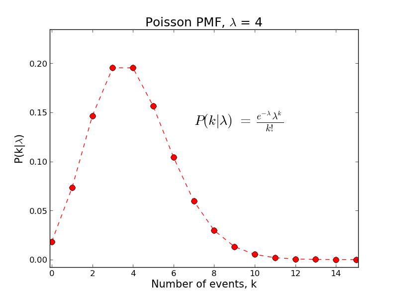
Related Entries:
Related Blog Posts:
A very closely related problem is analyzed by Allen Downey in this chapter from his book Think Bayes
Posterior Probability
A posterior probability distribution, often known simply as a posterior, is a probability distribution derived from Bayes' theorem. This means that it is a statement of the reliability of each of the propositions in some hypothesis space, based on prior information and some other additional knowledge.
When further additional information comes to light, a further implementation of Bayes' theorem can be performed, using the current posterior as the prior, thus generating a new posterior.
Related Entries:
Prior Probability
A prior probability distribution is a statement of probability derived from all the available prior information relevant to some set of hypotheses. The prior, as the this distribution is frequently known, is used as an input to Bayes' theorem.
Bayes' theorem converts a prior to a posterior distribution, meaning that additional information is combined with the prior information, resulting in an updated probability assignment. In subsequent iterations of Bayes' theorem, this posterior will assume the role of prior. Thus, the distinction between the prior information and the additional information to be incorporated using Bayes' theorem is arbitrary, and need not follow any strict historical order.
When first applying Bayes' theorem to some hypothesis-testing problem, the assignment of the prior requires additional technology, as there is no previous iteration of Bayes' theorem to call upon. One common method is the principle of indifference, which states that for a set of discrete hypotheses, all hypotheses must be assigned equal probability if there is no information to the contrary. This is a special case of a symmetry-based argument known as the principle of transformation groups. Another method of assigning the first prior to a problem is the principle of maximum entropy. When an initial prior is obtained in either of these ways, the result is termed an uninformative prior, since its assignment follows purely from the definition of the problem, and no other information.
Sometimes, for mathematical convenience (e.g. fulfilling the normalization requirement) a non-uninformative prior will be employed at the start of a problem. As long as reasonable care is taken, this is usually not a major problem, especially if the information content of the data being used to generate the posterior is moderately informative.
Related Entries:
Transformation Groups
Probability
Probability is a numeric measure of the reliability of propositions.
The measure of probability is characterized by the points of minimum and maximum reliability. The point of maximum reliability is fixed by Cox's theorems to be 1 (the sum rule). The point of minimum reliability is somewhat arbitrary, being constrained by Cox's theorems to being one of two possibilities: 0 or +∞. By universal conventional, 0 is chosen as the probability associated with a proposition whose falsity we can not be more confident of.
The probability for a proposition, A, is written P(A | B), where B is some proposition specifying the probability model and the information on which the assignment of probability is to be based. Expressions of the form P(A | B), in which the conditioning operator, "|", appears are sometimes referred to as conditional probabilities, but this terminology is redundant, as in reality, all probabilities are of this type (even though P(A) may sometimes be written as shorthand). This is an important point about probabilities: all probability assignments are contingent upon a probability model and some body of information. This is termed theory ladenness.
Note also that many programming languages use the symbol "|" to refer to disjunction. The expression "A|B" is thus used in such languages to test whether A or B (or both - this is entailed in the definition of 'or') are true. These two usages of "|" in probability and in programming have nothing in common.
In the absence of empirical data, probabilities can be assigned using at least two distinct methods: (1) symmetry and (2) the maximum entropy principle. The principle of indifference is a common example of the symmetry methods. Indifference recognizes that if nothing is known that makes one hypothesis in a given discrete hypothesis space more likely than any other, then it is inconsistent not to assign all hypotheses in that hypothesis space equal probability. If there are six hypotheses, therefore, as in the case of the outcome of rolling a six-side die, then the probability associated with each hypothesis is 1/6. The probability distribution resulting from such arguments are termed uninformative.
In the case where probabilities are to be calculated in light of more information-rich considerations (often a set of empirical data), Bayes' theorem can be used. An uninformative probability distribution may serve as the prior in this procedure, or the prior may be the result of a previous iteration of Bayes' theorem. The output of Bayes' theorem, the updated probability distribution, is termed the posterior.
Perfect knowledge is impossible. Consider an omniscient being. Such a being will necessarily perceive its own omniscience, yet there will be a difficulty if the being is to say with confidence whether or not that perception is illusory. There can be no algorithm for an omniscient being to solve this problem, and so there is something that the being does not know with certainty, and its omniscience is therefore an impossibility.
Absolute knowledge of the truth values of propositions about reality is typically impossible, therefore. The making of rational statements of knowledge is thus typically restricted to making statements of probability. When knowledge from empirical experience enters the process, then statements of knowledge are necessarily statements of probability, as the relationship between raw experience and reality can not be known with certainty.
In light of this, probability can be seen to form the basis for all science, and the theory of probability is therefore also the theory of scientific methodology. The scientific discipline of incorporating mathematically encoded observations into the pool of knowledge is often termed 'statistics'.
Related Entries:
principle of indifference
principle of transformation groups
maximum entropy principle
Theory Ladenness
principle of transformation groups
maximum entropy principle
Theory Ladenness
Related Blog Posts:
Total Bayesianism discusses the probabilistic basis for all science
The Calibration Problem: Why Science Is Not Deductive shows in detail why science necessarily relies on probabilities
The Calibration Problem: Why Science Is Not Deductive shows in detail why science necessarily relies on probabilities
Probability Distribution Function
A probability distribution function, f(x), is the mathematical specification of a probability distribution. Often this specification will take the form of an analytic expression.
The are two varieties of probability distribution function, depending on the nature of the hypothesis space. Each variety takes its name from the metaphorical association between probability and mass.
If the hypothesis is discrete, i.e. consisting of a countable number of non-connected propositions (such as A and A'), then the distribution function, f(x), is known as a probability mass function, or PMF. Each point in the hypothesis space has a value associated to it by f(x). These values are pure numbers, with no units - they are the probabilities. The normalization requirement, for example, is ensured by simply adding up all the values over all discrete points in the hypothesis space.
A continuous hypothesis space consists of an uncountably infinite number of hypotheses (even though the hypothesis space may extend over a finite domain). These hypotheses concern the possible values of some parameter, such as temperature, that can take any value over a continuous range.
With a continuous hypothesis space, the probability at a discrete point has no meaning. The best we can do is calculate the mass of probability in some infinitesimally narrow slice, from x to x + dx. This amount of probability is the area of a rectangle of width dx, and height f(x). Unit consistency demands, therefore, that the units of f(x) are 1/x. Extending the mass analogy, and noting that mass divided by space is termed 'density,' the distribution function, f(x), over a continuous hypothesis space is termed the probability density function, or PDF.
From the extended sum rule, the amount of probability mass associated with a composite hypothesis, a ≤ x ≤ b, is given by the integrating the PDF:
Important properties of a probability distribution function are its mean and standard deviation. When the results of an investigation are reported, these summary statistics are often all the information that is communicated. A typical example of this is a parameter estimate and its error bar.
The integral of a probability distribution function from -∞ to x, F(x), is termed the cumulative distribution function, or CDF.
Related Entries:
Product Rule
The product rule is a basic theorem of probability theory, specifying the probability for a conjunction, AB.
The rule is:
The rule is:
P(AB | C) = P(A | C) × P(B | AC)
The proposition AB evidently carries the same meaning as BA, and so the product rule can also be written:
P(AB | C) = P(B | C) × P(A | BC)
The product rule is one of three basic theorems, the other 2 being the sum rule, and the extended sum rule.
Related Entries:
Quantile Function
Given a probability distribution function over x and a given input p, from 0 to 1, the quantile function gives the value of x at which the cumulative probability is p. That is, it gives the value of x at which the CDF over x is equal to p. In other words, if the probability that X is equal to or less than some value is p, then the quantile function will return that value, when p is the input.
The quantile function is also known as the inverse cumulative distribution function. One can think of it as the result of taking the CDF then swapping the axes, and reflecting the curve through the diagonal:

Related Entries:
CDF
Back to top
Rationality
Rationality is behaviour aimed at maximizing the probability to attain one's goals.
Rationality is dependent on scientific method. Rationality consists of (a) forming a reliable model of reality so that (b) reliable predictions can be made about what actions are relatively likely to result in one's goals being achieved. (a) is instantly recognizable as science. Also, since science is the procedure of reliably answering questions of fact about reality, and questions about what will happen in the future under a certain set of circumstances are also questions of fact about reality, then (b) is also science.
Rationality is also intimately linked with morality. Since morality concerns how one ought to behave, and since it cannot be otherwise that moral facts are determined by one's goals, then rationality and morality are actually identical. It is immoral to be irrational, because morality concerns doing what one ought to do, which means doing what is called for in the pursuit of what is good, which entails doing the called-for groundwork, i.e. doing a rational analysis of the available evidence. Also, it is irrational to be immoral, since being immoral entails acting against what is desirable.
Not to behave rationally is an inconsistent mode of behaviour. To desire a thing is equivalent to desiring an efficient means to achieve it, meaning that to behave irrationally is to act as if you do not desire the things you desire.
Rationality is reflexive in several important ways. Firstly, in order to pursue one's goals, it is necessary to know what one's goals are. This can only be reliably addressed by rational investigation. Secondly, it is desirable to invest effort into examining the evidence that one's reasoning process is valid - it is rational to ask whether or not one's cognitive machinery is functioning well, and to study the common cognitive biases that affect agents like you. Thirdly (but by no means finally), it is rational to examine a credible estimate of whether or not a proposed rational procedure is worth the effort: if I desire a fun-filled life, it may not be rational to embark on a calculation expected to take at least 180 years to complete, in order to ascertain how best to achieve this. Rationally, our strategy must take account of the likely cost of our deliberations.
There is a distinction made sometimes (e.g. lesswrong.com) between epistemic rationality, concerned with attaining reliable beliefs about the world, and instrumental rationality, concerned with efficiently achieving one's desires, but these two can be seen to be identical. All instrumental rationality concerns successfully answering questions of fact concerning efficient strategy, and is thus also epistemic rationality. Also all epistemic rationality necessarily entails furthering ones goals, as any activity not expected to contribute to one's goals is irrational, thus all epistemic rationality is instrumental rationality.
One must be wary of concepts such as rigorous or complete rationality. These are crude idealizations with no real meaning. Rationality is critically dependent on knowledge of the real world, but such knowledge is always necessarily subject to uncertainty. This uncertainty can always be further managed, by collecting new data, or by adding complexity to one's probability model, via model comparison, but it can never be entirely eliminated. Any putative rigorous rationality would demand complete confidence in some procedure used to obtain complete confidence in an infinite regress of probability calculus. Thus, the best that rationalists can attain is reliable reasons not to doubt the results of their analyses. Hence the need for self-reflexivity, re-examination of assumptions, and regular updating based on new experience.
The best possible measure of a person's rationality, therefore, must be the extent to which they act according to beliefs that they have robustly reliable reasons to hold, or some similar formulation. Properly, then, rationality is not something black or white, but is something that we must, if acting coherently, seek to always improve upon. Detailed qualification of rationality is not impossible, but there are some problems with some of the current standards for doing this, as discussed in the next paragraph.
An entity that bases decisions on some rational algorithm is often termed a rational agent. Because rational decision making demands high quality inference (of types (a) and (b), above), rational agents employ probability theory, notably including Bayes' theorem. Psychologists, for example, sometimes also seek to rate a subject's rationality by assessing their closeness to 'Bayesian optimality'. This terminology is problematic, though. As noted above, due to the problem of theory ladenness, there is no final optimum of rationality, upon which no improvement can be made. Also, for the same reason, it is perfectly possible for two rational agents, with the same goals and exposed to identical experiences to produce different probability assignments and to behave differently. This is due to the non-uniqueness with which a probability model can be specified. Attempts to quantify the rationality of a set of different algorithms often forget this fact, leading to problems of interpretation, when it is claimed that one algorithm is more rational than an other, or that subject X is not a rational agent. It is not impossible to perform such comparisons meaningfully, but robust metrics of rationality will require careful thought and, critically, empirical verification.
Related Entries:
Related Blog Posts:
Science
Science is an educated attempt to gain insight into the structure of reality: its contents and the relationships between its component parts. It attempts to estimate what is true about nature. These goals are pursued using start-of-the-art knowledge and techniques.
From this definition, it is clear that science and philosophy have the same goals, and the same commitment to high-quality methodology, making them in fact really the same thing.
One thing that is implicit in the above definition, that is worth expressing explicitly, is the rejection of a possible alternative definition: "science is the activity of people called scientists." Science is not defined by who does the work, but by the quality of the resulting inferences. Nullius in verba, as the motto of a famous scientific society prescribes: on the word of nobody.
No knowledge of phenomena in the universe can be perfect, and so science is limited to ranking the plausibilities of propositions about such phenomena using probabilities. Rationality dictates, therefore, that Bayes' theorem, or equivalent techniques, are used when incorporating empirical observations into probability assignments concerning hypotheses about nature. This process of learning from experience is termed inductive inference.
The job of science is to make the best possible estimate of what is true. An important class of truths that science can investigate concerns the matter of how best to behave. Matters such as how to build a bridge that will not collapse, how to conduct science, and how to be a good person are all therefore contained within the broad discipline of science.
Related Entries:
Induction
Related Blog Posts:
Total Bayesianism
The Calibration Problem: Why Science Is Not Deductive shows in detail why science necessarily relies on probabilities
The Calibration Problem: Why Science Is Not Deductive shows in detail why science necessarily relies on probabilities
Sensitivity
Generally speaking, sensitivity is the capacity to register some actually occurring phenomenon. If something really exists, then a sensitive instrument is able to indicate its presence.
In statistics, the term is usually applied to a test that produces a binary outcome, such as whether or not a patient has a certain medical condition, whether or not some gene has mutated, or whether or not a particular building is on fire. In this case, the sensitivity of a test is the probability that the instrument will infer 'true' with respect to the variable under examination, given that the state of reality is 'true', in this regard.
Sensitivity is thus the ratio of true cases recognized as true to the total number of true cases examined, and can consequently be expressed in terms of the expected numbers of true positives and false negatives:

Given that the true positive rate and false negative rate sum to 1, the sensitivity can also be expressed in terms of the false negative rate only:
When designing an instrument, sensitivity must be considered together with specificity. It is trivially easy to devise an instrument whose sensitivity is 100 % (the alarm is constantly sounding), but then the specificity will necessarily be zero. The converse is also true, increasing specificity often leads to a worsening of the sensitivity. Design of an instrument with an appropriate decision point (sound the alarm if the density of smoke particles in the air exceeds x) depends, formally or informally, on decision theory and some inferred utility function.
Another term for the sensitivity of an experiment is statistical power.
In other situations, such as particle counting, sensitivity is referred to as efficiency.
Related Entries:
Utility
Specificity
Generally speaking, specificity is the ability of an instrument designed to register the presence of some phenomenon to remain in a non-activated state when the phenomenon is not present.
In statistics, the term is applied to a test that produces a binary outcome, such as whether or not a patient has a certain medical condition, whether or not some gene has mutated, or whether or not a particular building is on fire. The specificity of a test is the probability that the instrument will infer 'false' with respect to the variable under examination, given that the state of reality is 'false', in this regard.
Specificity is the ratio of false cases recognized as false (true negatives) to the total number of false cases examined, and can consequently be expressed in terms of the expected numbers of true negatives and false positives:

Given that the true negative rate and false positive rate sum to 1, the specificity can also be expressed in terms of the false positive rate only:

When designing an instrument, specificity must be considered together with sensitivity. It is straightforward to devise an instrument whose specificity is 100 % (the alarm is disconnected from the battery), but then the sensitivity will necessarily suffer. The converse is also true, increasing sensitivity often leads to a worsening of the specificity. Design of an instrument with an appropriate decision point (sound the alarm if the density of smoke particles in the air exceeds x) depends, formally or informally, on decision theory and some inferred utility function.
Related Entries:
Utility
Standard Deviation
The standard deviation of a set of numbers is the average distance of the numbers from the mean of the set. If a distribution is sampled at random, the standard deviation is the expected absolute value of the difference between the sample and the distribution's mean. The standard deviation of a probability distribution over x, denoted σ, is given by the formula:
σ2 = 〈x2〉 - 〈x〉2
where the angle brackets denote expectation.
The square of the standard deviation, appearing in the above formula, is referred to as the variance.
The standard deviation characterizes the dispersion of a probability distribution, meaning that it conveys information about the distribution's width. A wider distribution implies greater uncertainty.
The standard deviation of a sample of size N is calculated using the following formula, in which the over-bar denotes the sample mean:

Here, the Σ denotes summation over all N cases within the sample.
Related Entries:
Student's t-Distribution
Student's t-distribution is a sampling distribution used when the distribution associated with a random variable with an assumed, but unknown normal distribution is estimated from a small number of samples. It is a function, f(t, ν), of the t-parameter and a number of degrees of freedom, ν. The number of degrees of freedom (often denoted 'dof') is closely related to the number of samples, n, from which the distribution is estimated. The t-distribution has mean of zero, and is symmetric about its mean.
When the frequency distribution for a random variable is estimated, uncertainty exists as to the distribution's standard deviation, with the result that student distribution appears similar to the normal distribution, but with more probability mass in the tails of the distribution. The more samples are used to estimate the distribution, the closer it appears to the normal. Thus, in the limit as n approaches ∞, f(t, ν) → N(t | μ=0, σ = 1), the standard normal distribution. At the other end of the scale, ν = 1, the student distribution is the Cauchy distribution.
Student's distribution is very popular in frequentist hypothesis testing. When used in this setting, a t-parameter, t, is derived from a data set, and the significance of the result, i.e. how unexpected it is under the null hypothesis, is assessed by effectively measuring the distance of the obtained t-parameter from 0. This procedure is generally (independent of the sampling distribution) known as null-hypothesis significance testing. Specification of a p-value, however, requires integrating the tails of the t-distribution from ± t, outwards (two-tailed test).
For example, when the null hypothesis asserts that the mean of a frequency distribution is μ0, and a single set of n samples from that distribution is obtained, the t-parameter is calculated from

where x̄ is the sample average, s is the sample standard deviation, and the number of degrees of freedom is, as with many other cases, ν = n - 1. Integrating the tails of the t-distribution in order to assess statistical significance is known as a t-test
The t-distribution is important other areas of applied statistics, such as Bayesian spectral analysis.
Functions for evaluating and integrating the t-distribution are included in many mathematical software packages. For example, the graph below was created using the Python function scipy.stats.t.pdf(). An expression for the student distribution is:

The gamma function, Γ(x), is a generalization of the factorial operation, (x-1)!, allowing non-integer x, and has the innocent looking expression:

If you ever need to evaluate the gamma function, naive calculation of the integral turns out to be hellishly inefficient, but good numerical approximations have been found. The Lanczos approximation, is quite straightforward to implement, very efficient, and, as far as I can tell, the method used by most mathematical packages.
Plots of the t-distribution for several ν are shown below, and compared with the standard normal distribution:
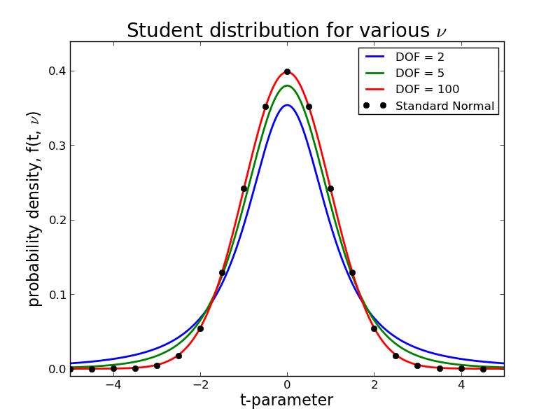
These plots give an impression of how many data points count as a 'small sample': with n - 1 = 100, the t-distribution is very close to normal.
The student distribution was first reported in 1908 by W.S. Gosset, who published under the pseudonym Student, reportedly to avoid difficulties associated with the intellectual property of his employer, Guinness Breweries.
Related Entries:
Probability Distribution Function
Normal Distribution
Null-Hypothesis Significance Test
Related Blog Posts:
I used the t-distribution in Signal and Noise
External Links:
W.S. Gosset, "The probable error of a mean," Biometrica 1908, vol 6, no. 1, pages 1-25, available here
Lanczos Approximation at wikipedia
Back to top
Sum Rule
The sum rule is a basic theorem of probability theory, specifying that the individual probabilities associated to a proposition, A, and its negation, A', add up to one, always.
Symbolically, this is written:
P(A) + P(A') = 1
This means that the maximum degree of confidence we can hold in a proposition is P = 1, and that any increase in confidence in a proposition must be matched by a decrease in confidence in its negation.
The sum rule is one of three basic theorems of probability theory, the other 2 being the product rule, and the extended sum rule.
Related Entries:
Survival Function
The survival function is the complement of the cumulative distribution function. That is, if the CDF is denoted F(x) and the survival function is denoted S(x), then
S(x) = 1 - F(x)
As F(x) is the probability that X is less than or equal to x, it follows that S(x) is the probability that X is greater than x,
S(x) = P(X > x).
We are often interested, however, in performing tails integrals of the form P(X ≥ x), which can be seen to be different to the survival function. For a discrete distribution, this tail integral can be obtained as S(x-1).
Related Entries:
PDFCDF
Back to top
Theory Ladenness
Theory ladenness is the condition that all probability assignments are dependent not only on prior information, but also on a set of assumptions, known as the probability model.
Given the central importance of probabilities in scientific method, the theory ladenness of probability entails the theory ladenness of science.
Failure to acknowledge the theory ladenness of probabilities is an example of the mind projection fallacy, in which elements of a model of reality are assumed to necessarily correspond to elements of reality.
Common examples of neglect of the theory ladenness of probabilities are unease with the practice of model checking, belief that probabilities equal to 0 or 1 should not take any part in rational deliberation, and many of the key beliefs within the frequency interpretation of probabilities.
Theory ladenness has negative associations for many, in major part, thanks to bad philosophers who have tried to argue that it entails that all points of view are equally valid.
Theory ladenness has negative associations for many, in major part, thanks to bad philosophers who have tried to argue that it entails that all points of view are equally valid.
Related Entries:
Model Checking
Related Blog Posts:
Inductive inference or deductive falsification?
Extreme values: P = 1 and P = 0
Back to top
XOR
XOR is a simple operation in Boolean logic. XOR is short for exclusive OR, where OR represents the logical disjunction.
XOR operates on two inputs (Boolean propositions) to yield a single Boolean output. The operation returns TRUE if exactly one of the inputs is TRUE, and FALSE otherwise.
The function XOR(A, B), also denoted A ⊕ B, has the following truth table:
| A | B | A ⊕ B |
| 0 | 0 |
0
|
| 0 | 1 |
1
|
| 1 | 0 |
1
|
| 1 | 1 |
0
|
Note that XOR(A, B) is distinct from OR(A, B), in that the latter also returns true if both inputs are true. In common usage, the word 'or' can refer to either the OR or XOR operations, but in rigorous parlance, no such flexibility is permitted.
A⊕B can be constructed in several ways using other basic Boolean operations, such as
A ⊕ B = (A + B) . ~(A . B)
No comments:
Post a Comment