The Ockham Factor

In an earlier post, I described how the method of maximum likelihood can deviate radically from the more logical results obtained from Bayes’ theorem, when there is strong prior information available. At the end of that post, I promised to describe another situation where maximum likelihood can fail to capture the information content of a problem, even when the prior distribution for the competing hypotheses is relatively uninformative. Having introduced the foundations of Bayesian model comparison, here, I can now proceed to describe that situation. I’ll follow closely a line of thought developed by Jaynes, in the relevant chapter from ‘Probability theory: the logic of science.’

In parameter estimation we have a list of model parameters, θ, a dataset, D, a model M, and general information, I, from which we formulate

(1)

P(D | θMI) is termed the likelihood function, L(θ | MDI) or more briefly, L(θ). The maximum likelihood estimate for θ is denoted.

When we have a number of alternative models, denoted by different subscripts, the problem of assessing the probability that the j^th model is the right one is just an equivalent one to that of parameter estimation, but carried out at a higher level:

(2)

The likelihood function here makes no assumption about the set of fitting parameters used, and so it decomposes into an integral over the entire available parameter space (extended sum rule, with P(H_iH_j) = 0, for all i ≠ j):

(3)

and the denominator is as usual just the summation over all n competing models, and so we get

(4)

In orthodox hypothesis testing, the weight that a hypothesis is to be given (P(H | DI) for us) is addressed with a surrogate measure: the likelihood function, which is what we would write as P(D | HI). Parameter estimation has never been considered in orthodox statistics to be remotely connected with hypothesis testing, but, since we now recognize that they are really the same problem, we can see that if the merits of two models, M_j and M_k are to be compared, orthodox statistics should do so by calculating the ratio of the likelihood functions at their points of maximum likelihood:

(5)

This, I admit, is something of a straw-man metric – I’m not aware if anybody actually uses this ratio for model comparison, but if we accept the logic of maximum likelihood, then we should accept the logic of this method. (Non-Bayesian methods that attempt to penalize a model for having excessive degrees of freedom, such as the adjusted correlation coefficient, exist, but seem to me to require additional ad hoc principles to be introduced into orthodox probability theory.) Let’s see, then, how the ratio in expression (5) compares to the Bayesian version of Ockham’s razor.

In calculating the ratio of the probabilities for two different models, the denominators will cancel out – it is the same for all models.

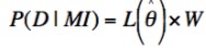
Lets express the numerator in a new form by defining the Ockham factor, W (for William, I guess), as follows:

(6)

which is the same as

(7)

from which it is clear that

(8)

Now we can write the ratio of the probabilities associated with the two models, M_j and M_k, in terms of expression (5):

(9)

So the orthodox estimate is multiplied by two additional factors: the prior odds ratio and the ratio of the Ockham factors. Both of these can have strong impacts on the result. The prior odds for the hypotheses under investigation can be important when we already had reason to prefer one model to the other. In parameter estimation, we’ll often see that these priors make negligible difference in cases where the data carry a lot of information. In model comparison, however, prior information of another kind can have enormous impact, even when the data are extremely informative. This is introduced by the means of the Ockham factor, which can easily overrule both the prior odds and the maximum-likelihood ratio.

In light of this insight, we should take a moment to examine what the Ockham factor represents. We can do this in the limit that the data are much more informative than the priors, and the likelihood function is sharply peaked at  (which is quite normal, especially for a well designed experiment). In this case, we can estimate the sharply peaked function L(θ) as a rectangular hyper-volume with a ‘hyper-base’ of volume V, and height . We choose the size of V such that the total enclosed likelihood is the same as the original function:

(10)

We can visualize this in one dimension, by approximating the sharply peaked function below by the adjacent square pulse, with the same area:

Since the prior probability density P(θ | MI) varies slowly over the region of maximum likelihood, we observe that

(11)

which indicates that the Ockham factor is a measure of the amount of prior probability for θ that is packed into the high-likelihood region centered on , which has been singled out by the data. We can now make more concrete how this amount of prior probability in the high likelihood region relates to the ‘simplicity’ of a model by noting again the consequences of augmenting a model with an additional free parameter. This additional parameter adds another dimension to the parameter space, which, by virtue of the fact that the total probability density must be normalized to unity, necessitates a reduction of magnitude of the peak of P(θ | MI), compared to the low-dimensional model. Lets assume that the more complex model is the same as the simple one, but with some additional terms patched in (the parameter sample space for the smaller model is embedded in that of the larger model).  Then we see that it is only if the maximum-likelihood region for the more complex model is far from that of the simpler model, that the Ockham factor has a chance to favor the more complex model.

For me, model comparison is closest to the heart of science. Ultimately, a scientist does not care much about the magnitude of some measurement error, or trivia such as the precise amount of time it takes the Earth to orbit the sun. The scientist is really much more interested in the nature of the cause and effect relationships that shape reality. Many scientists are motivated by desire to understand why nature looks the way it does, and why, for example, the universe supports the existence of beings capable of pondering such things. Model comparison lifts statistical inference beyond the dry realm of parameter estimation, to a wonderful place where we can ask: what is going on here? A formal understanding of model comparison (and a resulting intuitive appreciation) should, in my view, be something in the toolbox of every scientist, yet it is something that I have stumbled upon, much to my delight, almost by chance.