Great Expectations

Thinking ahead to some of the things I'd like to write about in the near future, I expect I'm going to want to make use of the technical concept of expectation. So I'll introduce it now, gently. Some readers will find much of this quite elementary, but perhaps some of the examples will be amusing. This post will be something of a moderate blizzard of equations, and I have some doubts about it, but algebra is important - it's the grease that lubricates the gears of all science. Anyway, I hope you can have some fun with it.

Expectation is just a technical term for average, or mean. It goes by several notations: statisticians like E(X), but physicists use the angle brackets, <X>. As physicists are best, and since E(X) is something I've already used to denote the evidence for a proposition, I'll go with the angle brackets.

We've dealt with the means of several probability distributions, usually denoting them by the Greek letter μ, but how does one actually determine the mean of a distribution? A simple argument should be enough to convince you of what the procedure is. The average of a list of numbers is just the sum, divided by the number of entries in the list. But if some numbers appear more than once in the list, then we can simplify the expression of this sum by just multiplying these by how often they show up. For n unique numbers, x₁, x₂, ..., x_n, appearing k₁, k₂, ..., k_n times, respectively, in the list, the average is given by

(1)

But if we imagine drawing one of the numbers at random from the list, the probability to draw any particular number, x_i, by symmetry is just k_i / (k₁+ k₂ + ... + k_n), and so the expectation of the random variable X is given by

(2)

In the limit where the adjacent points in the probability distribution are infinitely close to one another, this sum over a discrete sample space converts to an integral over a continuum:

(3)

In the technical jargon, when we say that we expect a particular value, we don't quite mean the same thing one usually means. Of course, the actual realized value may be different from what our expectation is, without any contradiction. The expectation serves to summarize our knowledge of what values can arise. In fact, it may even be impossible for the expected value to be realized - the probability distribution may vanish to zero at the expectation if, for example, the rest of the distribution consists of two equally sized humps, equally distant from <X>. (This occurs, for instance, with the first excited state of a quantum-mechanical particle in a box - such a particle in this state is never found at the centre of the box, even though that is the expectation for its position.) This illustrates starkly that it is by no means automatic that the point of expectation is the same as the point of maximum probability.

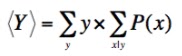
We can easily extend the expectation formula in an important way. Not only is it useful to know the expectation of the random variable X, but also it can be important to quantify the mean of another random variable, Y, equal to f(X), some function of the first. The probability for some realization, y, of Y is given by the sum of all the P(x) corresponding to the values of x that produce that y:

(4)

This follows very straightforwardly from the sum rule: if a particular value for y is the outcome of our function f operating on any of the x's in the sub-list {x_j, x_k, ...}, then P(y) is equal to P(x_j or x_k or ...), and since the x's, are all mutually exclusive, this becomes P(x_j) + P(x_k) + ....

Noting the generality of equation 2, it is clear that

(5)

which from equation (4) is

(6)

which by distributivity gives

(7)

and since all x map to some y, and replacing y with f(x), this becomes

(8)

which was our goal.

Suppose a random number generator produces integers from 1 to 9, inclusive, all equally probable, what is the expectation for x, the next random digit to come out? Do the sums, verify that the answer is 5. Now, what is the expectation of x²? Perhaps we feel comfortable guessing 25, but better than guessing, lets use equation (8), which we went through so much trouble deriving. The number we want is given by Σ(x²/9), which is 31.667. We see that <x²> ≠ <x>², which is a damn good thing, because the difference between these two is a special number: it is the variance of the distribution for x, i.e. the square of the standard deviation, which (latter) is the expectation of the distance of any measurement from the mean of its distribution. This result is quite general.

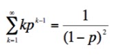
As another example, lets think about the expected number of coin tosses, n, one needs to perform before the first head comes up. The probability for any particular n is the probability to get 1 - n tails in a row, followed by 1 head, which is (1/2)ⁿ. We're going to need an infinite sum of these terms, each multiplied by n. There's another fair chunk of algebra following, but nothing really of any difficulty, so don't be put off. Take it one line at a time, and challenge yourself to find a flaw - I'm hoping you won't. I'll start by examining this series:

(9)

multiplying both sides by a convenient factor,

(10)

then removing all terms that annihilate each other, and dividing by that funny factor,

(11)

But p is going to be the probability to obtain a head (or a tail) on some coin toss, so we know it’s less than 1, which means that as n goes to infinity, pⁿ⁺¹ goes to 0, so

(12)

Now the point of this comes when we take the derivative of equation (12) with respect to p:

(13)

Finally, to bump that power of p on the left hand side up from k-1 to k, we just need to multiply by p again, which gives us, from equation (2), the expectation for the number of tosses required to first observe a head:

(14)

Noting that p = 1/2, we find that the expected number of tosses is a neat 2.

Perhaps you already guessed it, but I find this result quite extraordinarily regular. Of all the plausible numbers it could have been, 3.124, 1.583, etc., it turned out to be simple old 2. Quite an exceptionally well behaved system. Unfortunately, all the clunky algebra I've used makes it far from obvious why the result is so simple, but we can generalize the result with a cuter derivation that will also leave us closer to this understanding. We can do this using something called the theorem of total expectation:

(15)

It’s starting to look a little like quantum mechanics, but don’t worry about that. This theorem is both intuitively highly plausible and relatively easy to verify formally. I won't derive it now, but I'll use it to work out the expected number of trials required to first obtain an outcome whose probability in any trial is p. I'll set x equal to the number of trials required, n, and set y equal to the outcome of the first trial:

(16)

The expectation of n, when n is known to be 1 is, not surprisingly, 1. Not only that, but the expectation when n is known to be not 1 is just 1 added to the usual expectation of n since one of our chances out of all those trials has been robbed away: 

(17)

which is very easily solved,

(18)

So the result for the tossed coin, where p = (1 - p) = 0.5, generalizes to any value for p: the expected number of trials required is 1/p. 

Finally a head scratching example, not because of its difficulty (its the simplest so far), but because of its consequences. Imagine a game in which the participant tosses a coin repeatedly until a head first appears, and receives as a prize 2ⁿ dollars, where n is the number of tosses required. This famous problem is known as the St. Petersburg paradox. The expected prize is Σ(2ⁿ/2ⁿ), which clearly diverges to infinity. Firstly, this illustrates that not all expectations are well behaved. Further, the paradox emerges when we consider how much money we should be willing to pay for the chance to participate in this game. Would you be keen to pay everything you own for an expected infinite reward? Why not? Meditation on this conundrum led Daniel Bernoulli to invent decision theory, but how and why will have to wait until some point in the future.