Maximum Entropy: Calibrating an X-ray Spectrometer

Calibration is a process whereby a relationship is inferred between the output of some measuring instrument and the physical process responsible for that output. An instrument may be something as simple as a ruler, or something as complicated as the Human Genome Project or the Planck cosmic background survey. Calibration is fundamental to science. We might even say that it is science.

When we think about calibration, we often think simply about finding the most probable value for some physical parameter, given some reading from an instrument. In the previous part, I described this simple process for a device used to characterize the distribution of photon energies in a stream of x-rays.

But we really ought to think of calibration as more than this. To make the best inferences possible from a reading, we should formulate the entire probability distribution, not just the location of its maximum, for the state of the world when the machine goes "bing," or when the display reads "42." When the readout says 7, it's good to know that I've most probably just found a black hole (perhaps), but it's also good to know what alternative explanations there are, and what amounts of probability mass they command.

At the end of the previous post, I showed this measurement of an x-ray spectrum, made with a cadmium telluride (CdTe) detector:

As I explained, those step-like drops in intensity at 27 and 32 keV are artifacts of the detector, and are consequences of an asymmetric probability distribution, P(state of the world | this instrument reading). Such asymmetry makes it all the more important to look beyond determining just the distribution's peak, as it means that our instrument is systematically distorting the truth. In this post, I'll describe my analysis aimed at converting this repeatably distorted detected spectrum to a representation of the true spectrum of the source.

The detector, of course, is made of atoms (Cd and Te), and these atoms have K-edges just like all others, as I described previously. That means that when a photon with more energy than these K-edges is absorbed, there is a chance for a fluorescence photon to leave the detector, taking away its characteristic energy with it. This energy, of course, does not contribute to the number of photo-generated electrons in the current pulse corresponding to such a detection event, and the detector registers photons with systematically lower energy than they really have. The two steps in the spectrum correspond to the points at which the incoming photons first exceed the Cd and Te K-edges. Every time a fluorescence photon escapes, the registered energy equals the true energy minus that of the fluorescence photon.

We want to work out the probability for a K-photon to escape the detector, so we can correct this asymmetric distortion. Let’s start by defining a few propositions:

A	≡	an x-ray photon from the source was absorbed in the detector

Cd	≡	an x-ray was absorbed by a cadmium atom in the detector

z	≡	an x-ray from source was absorbed at depth = z

E	≡	a fluorescence photon escaped the detector

K	≡	a K-shell emission occurred

K_i	≡	a K-shell emission into the i^th recombination channel occurred

θ	≡	a fluorescence photon was emitted at angle θ, with respect to the optic axis

E_i	≡	a fluorescence photon from the i^th recombination channel escaped the detector

D	≡	an absorbed photon from the source is detected in full (the full amount of energy absorbed is converted to charges collected at the readout electrode)

In the derivation below, I'll only consider the case where a photon is absorbed by a cadmium atom, but the full calculation will consist of also examining the alternate case, where absorption occurs in tellurium. For this, we just need to replace P(Cd | A, I) with P(Te | A, I) = 1 - P(Cd | A, I), from the sum rule.

We want to know the number of x-ray photons absorbed in the detector, N_A. What we actually know is the number detected, N_D.

On average, the number detected is

Once a photon has been absorbed, our probability model, I, assumes that the only possibility for it to be not detected in full is for some of the energy to escape as a fluorescence photon. Thus, from the sum rule,

Also, our model assumes exactly 4 fluorescence channels:

i	channel	fluorescence energy (keV)
1	Cd, K_α	23.2082
2	Cd, K_β	26.1586
3	Te, K_α	27.3773
4	Te, K_β	31.091

So, the detection probability is

Or, invoking the extended sum rule for disjoint propositions,

From which, we can estimate the number of absorbed x-rays from the number detected:

(1)

A fluorescence photon can only escape the detector if it has been emitted, so the proposition E_i is the same as the proposition E_i K_i. Thus,

which, from the product rule, can be decomposed:

(2)

The probability for K-emission in the i^th channel can also be similarly decomposed. For example, for i = 1, K_α emission from cadmium, K₁ is a conjunction of three things: (a) absorption by a cadmium atom, (b) emission of a fluorescence photon (i.e. no non-radiative relaxation, such as Auger recombination, where the energy goes into another electron), and (c) emission into the α line:

The first term is the relative intensity (material dependent) of the K_α line, obtainable from published tables,

The second term is the overall K-fluorescence yield, termed ω_K, obtained from literature¹, and the third term is given by the photoelectric absorption coefficients (discussed two posts ago):

We need one other term in order to evaluate Eq. (2). The escape probability is dependent on the unknown absorption depth, z, of the incident x-ray photon. We will integrate this nuisance parameter out, to give the desired marginal distribution:

The absorption depth is independent of the ensuing fluorescence channel, so

(3)

Note that, from the product rule,

i.e. the probability to be absorbed at a given depth (obtained from the exponential distribution) must be normalized by dividing by the overall absorption probability in the 1 mm thickness of the detector.

The depth-dependent escape probability, P(E_i | z, K_i, A, I), is also dependent on the unknown emission angle of the fluorescence photon, θ, relative to the direction of travel of the detected photon (perpendicular to detector surface). This is because different angles (for a given emission depth) correspond to different distances required to exit the CdTe detector. Again, let’s marginalize over this nuisance parameter:

(4)

(θ is independent of all other variables, and is uniform over 0 ≤ θ ≤ π, hence P(θ | I) × dθ is 1 divided by the number of samples over the half circle.)

Strictly, we should integrate over two angles, θ and φ (the detector has a square profile, and escape distances from the side depend on φ), but because the detector is heavily masked, so that only the centre is illuminated, and because the detector is very wide, compared to the penetration depth at the K-photon energies, we treat escape from the bottom or top as the only escape paths. This is supported by noting that reducing the size of the mask aperture has no effect on these observed artifacts. For the same reason, my model does not integrate over the x- and y-coordinates in the detector volume.

For emission angles less than 90⁰ (moving downwards), the distance required to exit the detector through the bottom surface is

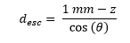
while for photons moving upwards, the distance to escape through the top is

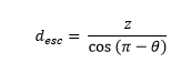
For each angle, and each depth, the desired escape probability is the exponential function: exp(-µ_PE × d_esc), where µ_PE is the photo-electric absorption coefficient at the relevant energy.

Finally, combining Eq’s (2), (3), and (4), for the Cd K_α fluorescence channel, we have (with similar formulae for the other channels):

(5)

Using Eq’s (5) and (1), we can get the number of photons absorbed at each energy, from the number counted by the detector. The intensity at the j^th energy, I_j, needs to be enhanced according to Eq. (1). The intensities at each of the depleted energies, I_{j - n}, where n is the number of detector channels spanned by the energy of the relevant fluorescence photon, need to have a number of counts, I_j × P(E_i | A, I), subtracted.

The procedure starts at the highest energy in the spectrum. Once the j^th detector channel has been processed, we move on to the j-1^th, until all channels have been adjusted. By traversing backwards through the spectrum, any contribution from higher energies will have been removed before the number of escape photons is calculated for each energy channel.

Note that the fluorescence yields are step functions of the incident energy – nothing is emitted for incident energies below the K-edges.

Once the detected spectrum has been converted to an absorbed spectrum, the spectrum incident on the detector is obtained by dividing the absorbed spectrum by the energy-dependent quantum efficiency of the 1 mm CdTe detector, and finally, the spectrum incident on the outer window of the detector is obtained by dividing again, by the transmission efficiency of the 250 µm beryllium window. This allows characterization of the spectrum emitted by the source, which is the ultimate goal of the activity. These transmission and absorption efficiencies are obtained again, using the appropriate energy-dependent attenuation coefficients, all of which can be obtained from this convenient NIST database.

All the calculations I described were carried out by my computer. I numerically integrated over z, taking 200 samples, and θ, with 180 samples (taking care not to let θ = 90, to avoid division by zero when the cosine is taken). The result is as follows, and exhibits partial success:

It seems to me that all the logic I described is correct. All the simplifying assumptions seem reasonable, and I have checked the code and not found any errors, but sadly, the result is not quite what it should be. Those spurious steps in the spectrum have been successfully removed, but have been replaced by a couple of sharp spikes. Evidently my model of the device is not quite adequate. These spikes could relatively easily be removed, by simply noting that they shouldn't be there - they are narrow enough that a linear or quadratic interpolation between the points on either side would be a fair fix, though a highly unsatisfying one. There's still some work to do here, before total victory can be declared.

In the literature, I see others working with a similar spectrometer encountered similar difficulties, which they also couldn't explain². Here is my best (though at present, highly speculative) guess for what might be happening:

My model assumes the onset of the K-edge is immediate, in line with basic known physics. But the original spectrum shows a gradual onset over almost 2 keV. Naturally, the detector exhibits measurement uncertainty in the form of a symmetric broadening, but at < 0.2 keV (known from the fluorescence measurements) this is insufficiently broad to account for the observed effect. The detector, however, is placed under a high voltage, to drive the photo-generated electrons to the readout electrode - several hundred volts, which results in a strong electric field that could conceivably affect measurably the binding energies of the atoms' electrons. Furthermore, CdTe technology is not as well developed as that of other semiconductors, such as silicon, and the CdTe crystals that can be grown are not of such high quality. Because of this, defects in the CdTe crystal can lead to local and transient distortion of the applied electric field, which just might lead to small differences in the effective K-edges at different locations (and different times). There could be some really interesting device physics going on here. If so, remember, you heard it here first!

If I make significant progress with this, I'll try to post a follow-up. If you know how to solve this problem, please drop me an email!

References

[1]	A. Markowicz, in Handbook of X-Ray Spectrometry, edited by Van Grieken and Markowicz, (Marcel Dekker) 2002
[2]	R. Redus, J. Pantazis, T. Pantazis, A. Huber, and B. Cross, Characterization of CdTe detectors for quantitative X-ray spectroscopy, presented at the 2007 Denver X-ray Conference and submitted to IEEE Trans. Nucl. Sci, 2008