The Ockham Factor

In an earlier post, I described how the method of maximum likelihood can deviate radically from the more logical results obtained from Bayes’ theorem, when there is strong prior information available. At the end of that post, I promised to describe another situation where maximum likelihood can fail to capture the information content of a problem, even when the prior distribution for the competing hypotheses is relatively uninformative. Having introduced the foundations of Bayesian model comparison, here, I can now proceed to describe that situation. I’ll follow closely a line of thought developed by Jaynes, in the relevant chapter from ‘Probability theory: the logic of science.’

In parameter estimation we have a list of model parameters, θ, a dataset, D, a model M, and general information, I, from which we formulate

(1)

P(D | θMI) is termed the likelihood function, L(θ | MDI) or more briefly, L(θ). The maximum likelihood estimate for θ is denoted.

When we have a number of alternative models, denoted by different subscripts, the problem of assessing the probability that the j^th model is the right one is just an equivalent one to that of parameter estimation, but carried out at a higher level:

(2)

The likelihood function here makes no assumption about the set of fitting parameters used, and so it decomposes into an integral over the entire available parameter space (extended sum rule, with P(H_iH_j) = 0, for all i ≠ j):

(3)

and the denominator is as usual just the summation over all n competing models, and so we get

(4)

In orthodox hypothesis testing, the weight that a hypothesis is to be given (P(H | DI) for us) is addressed with a surrogate measure: the likelihood function, which is what we would write as P(D | HI). Parameter estimation has never been considered in orthodox statistics to be remotely connected with hypothesis testing, but, since we now recognize that they are really the same problem, we can see that if the merits of two models, M_j and M_k are to be compared, orthodox statistics should do so by calculating the ratio of the likelihood functions at their points of maximum likelihood:

(5)

This, I admit, is something of a straw-man metric – I’m not aware if anybody actually uses this ratio for model comparison, but if we accept the logic of maximum likelihood, then we should accept the logic of this method. (Non-Bayesian methods that attempt to penalize a model for having excessive degrees of freedom, such as the adjusted correlation coefficient, exist, but seem to me to require additional ad hoc principles to be introduced into orthodox probability theory.) Let’s see, then, how the ratio in expression (5) compares to the Bayesian version of Ockham’s razor.

In calculating the ratio of the probabilities for two different models, the denominators will cancel out – it is the same for all models.

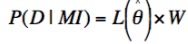
Lets express the numerator in a new form by defining the Ockham factor, W (for William, I guess), as follows:

(6)

which is the same as

(7)

from which it is clear that

(8)

Now we can write the ratio of the probabilities associated with the two models, M_j and M_k, in terms of expression (5):

(9)

So the orthodox estimate is multiplied by two additional factors: the prior odds ratio and the ratio of the Ockham factors. Both of these can have strong impacts on the result. The prior odds for the hypotheses under investigation can be important when we already had reason to prefer one model to the other. In parameter estimation, we’ll often see that these priors make negligible difference in cases where the data carry a lot of information. In model comparison, however, prior information of another kind can have enormous impact, even when the data are extremely informative. This is introduced by the means of the Ockham factor, which can easily overrule both the prior odds and the maximum-likelihood ratio.

In light of this insight, we should take a moment to examine what the Ockham factor represents. We can do this in the limit that the data are much more informative than the priors, and the likelihood function is sharply peaked at  (which is quite normal, especially for a well designed experiment). In this case, we can estimate the sharply peaked function L(θ) as a rectangular hyper-volume with a ‘hyper-base’ of volume V, and height . We choose the size of V such that the total enclosed likelihood is the same as the original function:

(10)

We can visualize this in one dimension, by approximating the sharply peaked function below by the adjacent square pulse, with the same area:

Since the prior probability density P(θ | MI) varies slowly over the region of maximum likelihood, we observe that

(11)

which indicates that the Ockham factor is a measure of the amount of prior probability for θ that is packed into the high-likelihood region centered on , which has been singled out by the data. We can now make more concrete how this amount of prior probability in the high likelihood region relates to the ‘simplicity’ of a model by noting again the consequences of augmenting a model with an additional free parameter. This additional parameter adds another dimension to the parameter space, which, by virtue of the fact that the total probability density must be normalized to unity, necessitates a reduction of magnitude of the peak of P(θ | MI), compared to the low-dimensional model. Lets assume that the more complex model is the same as the simple one, but with some additional terms patched in (the parameter sample space for the smaller model is embedded in that of the larger model).  Then we see that it is only if the maximum-likelihood region for the more complex model is far from that of the simpler model, that the Ockham factor has a chance to favor the more complex model.

For me, model comparison is closest to the heart of science. Ultimately, a scientist does not care much about the magnitude of some measurement error, or trivia such as the precise amount of time it takes the Earth to orbit the sun. The scientist is really much more interested in the nature of the cause and effect relationships that shape reality. Many scientists are motivated by desire to understand why nature looks the way it does, and why, for example, the universe supports the existence of beings capable of pondering such things. Model comparison lifts statistical inference beyond the dry realm of parameter estimation, to a wonderful place where we can ask: what is going on here? A formal understanding of model comparison (and a resulting intuitive appreciation) should, in my view, be something in the toolbox of every scientist, yet it is something that I have stumbled upon, much to my delight, almost by chance.   

Ockham's Razor

Numquam ponenda est pluralitas sine necessitate.

- attributed to William of Ockham, circa 1300.

Translation: “Plurality should not be posited without need.”

The above quotation is understood to be a heuristic principle to aid in the comparison of different explanations for a set of known facts.

The principle is often restated as:

          ‘The simplest possible explanation is usually the correct explanation.’

This idea is frequently invoked by scientists, engineers, or any other class of person involved in rational decision making, very often without thinking. We know instinctively, for example, that when trying to identify the cause of the force between two parallel current-carrying wires, it is useless to contemplate the presence of monkeys on the moon. But this is the most trivial form of application of the Ockham principle, specifying our preferred attitude to entities of no conceivable relevance to the subject of study.

Less trivial applications occur when we contemplate things that would have an effect on the processes we study. In such cases it is still widely and instinctively accepted that we should postulate only sufficient causal agents to explain the recorded phenomena. We tend to see the ‘simplicity’ of an explanation, therefore, to be advantageous. Mathematically, this is related to the complexity of the mathematical model with which we formulate our description of a process.  A linear response model, for example, when it gives a good fit, is seen as more desirable than a quadratic model. This may be partly related to the greater ease with which a linear model can be investigated mathematically, but there is also a feeling that if the fit is good, then the linear model probably is the true model, even though the quadratic model will always give a better fit (lower minimized residuals) to noisy data.

Two problems arise if we try to make the Ockham principle objective:

(i)               How do we define the ‘simplicity’ of a model?

(ii)              How are we to determine when it is acceptable to reject a model in

                   favor of one less simple?  

A slightly loose definition of the simplicity of a model is the ease with which it can be falsified. That is, if a model makes very precise predictions, then it is potentially quickly disproved by data, and is considered simple. With a Bernoulli urn, for example, known to contain balls restricted to only 2 possible colours, the theory that all balls are the same colour is instantly crushed, if we draw 2 balls of different hues. An alternate model, however, that the urn contains an equal mixture of balls of both colours is consistent with a wider set of outcomes – if we draw 10 balls, all of the same colour, then it is less likely, but still possible that that there are balls of both colour in the urn.

To make the definition of simplicity more exact, we can say that the simpler model has a less dispersed sampling distribution for the possible data sets we might get if that model is true. P(D | M, I) is more sharply concentrated.

Mathematical models of varying numbers of degrees of freedom can also succumb to a characterization of their relative simplicity using this definition. If one finds that a simple model does not exactly fit the data, then one can usually quite easily ‘correct’ the model by adding some new free parameter, or ‘fudge factor.’ Adding an additional parameter gives the model a greater opportunity to reduce any discrepancies between theory and data, because the sampling distribution for the data is broader – the additional degree of freedom means that a greater set of conceivable observations are consistent with the model, and P(D | M, I) is spread out more thinly. This, however, means that it is harder to falsify the model, and it is this fact that we need to translate into some kind of penalty when we calculate the appropriateness of the model.

To see how we can use Bayes’ theorem to provide an objective Ockham’s razor, I’ll use a beautiful example given by Jeffreys and Berger¹, in ‘Sharpening Ockham’s Razor on a Bayesian Strop.’ The example concerns the comparison of competing theories of gravity in the 1920s: Einstein’s relativity, which we denote by proposition E, and a fudged Newtonian theory, N, in which the inverse-square dependence on distance is allowed instead to become d^-(2+ε), where ε is some small fudge factor. This was a genuine controversy at that time, with some respected theorists refusing to accept relativity. 

The evidence we wish to use to judge these models is the observed anomalous motion of the orbit of Mercury, seen to differ from ordinary Newtonian mechanics by an amount, a = 41.6 ± 2.0 seconds of arc per century. The value, α, calculated for this deviation using E was 42.9’’, a very satisfying result, but we will use our objective methodology to ascertain whether in light of this evidence, E is more probably the truth than N, the fudged Newtonian model. In order to do this we need sampling distributions for the observed discrepancy, a, for each of the models.

For E, this is straightforward (assuming the experimental error magnitude is normally distributed):

For N, the probability to observe any particular value, a, depends not only on the experimental uncertainty, σ, but also on the sampling distribution for α, the predicted value for the anomalous motion. This is because α is not fixed, due to the free parameter, ε. We can treat α as a nuisance parameter for this model:

To find P(α | N), we note that a priori, there is no strong reason for the discrepant motion to be in any given direction, so positive values are as likely as negative ones. Also large values are unlikely, otherwise they would be manifested in other phenomena. From studies of other planets, a value for α > 100’’ can be ruled out. Therefore, we employ another Gaussian distribution, centered at zero and with standard deviation, τ, equal to 50’’.

P(a | N) can then be seen to be a Gaussian determined by the convolution of the measurement uncertainty and the distribution for α:

We’ll consider ourselves to be otherwise completely ignorant about which theory should be favored, and assign equal prior probabilities of 0.5.

Bayes’ theorem in this case is:

and so we get the posterior probabilities: P(E | a, I) = 0.966 and P(N | a, I) =  0.034, which is nearly 30 times smaller. Because the fudged Newtonian theory has 2 uncertainties, the measurement error, and the free parameter, ε, the sampling distribution for the possible observed discrepancy, a, is spread over a much broader range.

Plotting the sampling distributions for the observed value, a, for each of the two models reveals exactly why their posterior probabilities are so different:

Because E packs so much probability into the region close to the observed anomaly, it comes out far more highly favored than N. If the actual observation was far from 40’’, then the additional degree of freedom of model N would be seen to be vindicated.

We can perform a sensitivity analysis to see whether we would have had a radically different result upon choosing a slightly different value for τ. Plotted below are the results for the same probability calculation just performed, but with a large range of possible values of τ:

The result shows clearly that we are not doing a great disservice to the data by arbitrarily setting τ at 50’’. The total absolute variation of P(E | a, I) is less than 0.04. We can also experiment with the prior probabilities, but remarkably, the posterior probability for the Einstein theory, P(E | a, I) falls only to 0.76 if P(E | I) is reduced to 0.1. This illustrates the important point that as long as our priors are somehow reasonably justified, the outcome is very often not badly affected by the slight arbitrariness with which they are sometimes defined.

Note that in order for the posterior probability, P(E | a, I), to be lowered to 0.5, the same value as the prior, we would need to increase the experimental uncertainty, σ, to more than 1000’’. This gives some kind of measure of the large penalty paid by introducing one extra free parameter.

The Ockham principle is a vague rule of thumb that, as we've just seen, can be derived from a much more general and quantitative principle, namely Bayes’ theorem. The fact that many people have been intuitively able to appreciate the validity of Ockham’s razor for roughly seven centuries is suggestive of how close Bayes’ theorem is to the way that human brains perform plausible reasoning. And why should it be any different? Bayes’ theorem is derived from robust logical principles, and it is no surprise that natural selection might favor information processing algorithms that mimic those principles.

In its original informal statement, Ockham’s razor may let us down in some cases, where there is strong prior information, where the ‘simplicity’ of two models is difficult to compare using our ill-defined, intuitive understanding of the term, or where the balance between goodness of fit and the penalty for complexity is too close for intuition alone to judge. The more general application of plausible reasoning using Bayes’ theorem, however, provides the best possible quality of inference, allows all these hard-to-define qualities (prior belief, simplicity, goodness of fit) to be objectively quantified, and puts model comparison on a firm logical basis.

---

[1] W.H. Jeffreys and J.O. Berger, ‘Sharpening Ockham’s Razor on a Bayesian Strop,’ Purdue University technical report #91-44C, August 1991 (Download here.)

The Higgs Boson at 5 Sigmas

Huge congratulations to Peter Higgs and the other theorists who, half a century ago, predicted this particle as part of the standard model, and to the experimentalists at CERN involved in making this recent discovery. We now have extremely compelling evidence of a new particle (new to us, at least) consistent with the Higgs boson. 

Sadly, there's much confusion circulating about the meaning of the 5σ significance level reported for the data on the Higgs. Lets first clear up what this means, before examining some of the confusion.

The null hypothesis, which states that there is no signal present in the data, only noise, implies that the magnitude for some parameter, Y, is some value, μ. Since there is random noise in the data, however, the value of Y observed in a measurement is unlikely to be exactly μ, but will follow a probability distribution with mean μ, and standard deviation σ. If the null hypothesis is true, then we can expect a measurement of Y to produce a result close to μ. The probability is less than 6 × 10^-7 that a measured value will be 5 standard deviations or further from μ, assuming the null hypothesis is true. This number is the p-value associated with the measurement. (In fact, for this case, a single-tailed test was performed, so the reported p-value for the Higgs boson is half this, about 2.8 × 10^-7.)

To recap, the reported p-value is the probability to observe data as extreme as or more extreme than than the data observed, assuming the null hypothesis is true. Roughly speeking, the p-value is P(D | H₀). David Spiegelhalter, over at the Understanding Uncertainty blog, has been monitoring press reports on the recent Higgs announcement, finding a high degree of misunderstanding among the journalists. Many writers described the reported p-value as the probability that the null hypothesis is true, calculated from the data, but this is P(H₀ | D), a very different thing, as I have described before.

Spiegelhalter has found numerous examples of this error, including writers from New Scientist and Nature, who really ought to know better. These are presumably professional journalists, however, who can perhaps be granted some slack, but what about a renowned cosmologist? How about these words:

Each experiment quotes a likelihood of very close to “5 sigma,” meaning the likelihood that the events were produced by chance is less than one in 3.5 million. 

These words come from Lawrence Krauss, a highly respected theoretical physicist, and they are wrong. I mentioned in my very first blog post that physicists are not generally so great at statistics, but I really don't like being proven right so blatantly. I suppose we really mustn't feel too bad about the mistakes in the press, when the experts can't get it right either.

In the article linked above, Spiegelhalter praises a couple of writers for getting the meaning of the p-value the right way round, but really these authors also fail to properly understand the matter. The passages, respectively from the BBC and from the Wall Street Journal, were:

...they had attained a confidence level just at the "five-sigma" point - about a one-in-3.5 million chance that the signal they see would appear if there were no Higgs particle.

and

If the particle doesn't exist, one in 3.5 million is the chance an experiment just like the one announced this week would nevertheless come up with a result appearing to confirm it does exist. 

While both these passages deserve praise for recognizing the p-value as the probability for the data, rather than the probability for the null hypothesis, they unfortunately are still not correct, for a reason that will bring me neatly in a moment to my second major point about the standard of reporting results such as these in terms of p-values. The reason these passages are wrong is that they employ an overly restrictive interpretation of the null hypothesis. They assume H₀ is the same as '"the Higgs boson does not exist," whereas the true meaning is broader: "there is no systematic cause of any patterns present in the data." If we reject the null hypothesis, we still have other possible non-Higgs explanations to rule out before we are sure that the Higgs boson is not a fantasy. These alternatives include other particles, consistent with different physical models; systematic errors in the measurements; and scientific fraud.

This might seem like a subtlety not really worth complaining about, but along with the other errors mentioned, it is a perpetuation of the fallacies surrounding the frequentist hypothesis tests - fallacies that mask the fact that the p-value is a poor summary of a data set, as I have explained in The Insignificance of Significance Tests. Why, for example, is it considered so important to rule out the null hypothesis so comprehensively, when there is little or no attempt to quantify the other alternative hypotheses? The possibility that the observation is a new particle, but not the Higgs, will no doubt be investigated substantially, but presumably will never be presented as a probability. The probability for fraud or systematic error will presumably receive absolutely no formal quantification at all.

Recently, we had a good example of how calculating the probability for measurement error could have prevented substantial trouble. As Ted Bunn has explained, it was a simple matter to estimate this quantity when researchers publicized results suggesting superluminal velocities for neutrinos, yet several groups set up experiments to try to replicate those result, at significant expense, despite the obviousness of the conclusion.

The traditional hypothesis tests set out to quantify, in a rather backwards way, the degree of belief we should have in the null hypothesis, but this is not what we are really interested in. What we want to know when a we look at the results of a scientific study is: what is the probability that the hypothesized phenomenon is real? For this, we should calculate a posterior probability. To do this, we need a specified hypothesis space with an accompanying prior probability distribution. This is one of the things that leads to great discomfort among some statistical thinkers, and was instrumental in leading to the adoption of the p-value as the standard measure of an experiment: how can you obtain a porsterior probability without violating scientific objectivity? How can you assign a prior probability without introducing unacceptable bias into the interpretation of the observations?

The people who think like this, though, don't seem to realize that prior probabilities can be assigned in a perfectly rigorous mathematical way, that will not introduce any unwarranted, subjective degree of belief. There seems to be a feeling like 'we don't know enough to specify the prior probability correctly,' but this is ridiculous - missing knowledge is exactly what probability theory is for. Any probability is just a formally derived, distilled summary of existing information. To calculate the probability for the Higgs, in principle all you need to do is start with a non-informative prior (e.g. uniform), figure out all the relevant information, and bit by bit account for each piece of information using Bayes' theorem. Sure, the bit about figuring out the relevant information is hard, but all those clever particle physicists at CERN must be able, if they put their minds to it. Then it is just a matter of investigating how well the various hypotheses, with and without the Higgs boson, account for various observations, and how efficiently they do so. We'll get a glimpse of how this is done, in a future post, when I get around to discussing model comparison, and a formal implementation of Ockham's razor.

Yes, there will always need to be assumptions made, in order to carry out such a program, but inductive inference is impossible without assumptions, (if you don't believe me, try it!) and any competent scientist (almost by definition) will be able to keep the assumptions used to those that either are accepted by practically everybody, or make negligible difference to the result of the calculation. It is the frequentists who are committing a fallacy by trying to learn in a vacuum.

I find it a great pity that the posterior distribution was not the chosen route taken for reduction of the data from the Large Hadron Collider. Firstly, this is an extremely fundamental question, and if any question deserves the best possible answer from the available data, this is it. The p-value simply doesn't extract all the information from the observations we now have at our disposal. Secondly, yes: it is a hugely complicated problem to assign a prior probability to a hypothesis like this, but this is a project involving a huge number of presumably some of the finest scientific minds around - if anybody can do it, they can. If they did, it would first of all prove that it can be done, and secondly it would lay a very strong foundation for the development of general techniques and standards for the computation of all manner of difficult-to-obtain priors.

The Mind Projection Fallacy

There is an argument that I have noted a couple of times when scientific colleagues with religious beliefs have tried to explain to me how they reconcile these seemingly contradictory things. Reality, they say, is divided into two classes of phenomena: the natural and the supernatural. Natural phenomena, they say, are the things that fall into the scope of science, while the supernatural lies outside of science’s grasp, and can not be addressed by rational investigation. This is completely muddle-headed, and seems to me to be based on an example of something called the mind projection fallacy.

A similar argument also crops up occasionally when advocates of alternative medicine try to rationalize the complete failure of their favorite pseudoscientific therapy to provide any evidence of efficacy in rigorous trials.

The very word ‘supernatural,’ at its heart, though, is one of those utterly self-defeating terms, like ‘free will’ and ‘alternative medicine,’ completely devoid of meaning and philosophically bankrupt. What is this free will that people keep going on about? Is it the freedom to break the laws of physics? No, and since every particle in your brain obeys the laws of physics, you are not free to make non-mechanistic decisions, so can we please shut up about free will? (Granted, I am using a restricted meaning of the term ‘free will.’)

And what is alternative medicine? Medicine is the use of interventions that are known to work in order to lessen the effects of disease. If it doesn’t work, or is not known to work, then its not medicine, full stop. There is no alternative. Lets please shut about alternative medicine.

What is the supernatural? Nature is by definition everything that exists and happens. What is outside nature is therefore necessarily an empty set.

The etymology of the word ‘supernatural’ is the result of an error of thinking. This error is the mind projection fallacy: falsely assuming that the properties of one’s model of reality necessarily exhibit correspondence with the actual properties of reality. The following dictionary definition of ‘supernatural’ was quoted to me in a recent discussion of the term (reportedly from Webster’s):

Supernatural. [adjective:] 1. of, pertaining to, or being ‘above or beyond what is natural or explainable by natural law’. 2. of, pertaining to, or attributed to God or a deity. 3. of a superlative degree; preternatural. 4. pertaining to or attributed to ghosts, goblins, or other unearthly beings; eerie; occult.

Number 1, is where we have to focus. Numbers 2 and 4 are, in origin at least, based on erroneous application of number 1, while number 3 is just weird. ‘Of a superlative degree’? That’s not supernatural, by any reasonable standard. ‘Preturnatural’? This word has two meanings (according to Dictionary.com): one is ‘supernatural’ (wow, that’s helpful) and the other is ‘exceptional or abnormal.’ Finding a hundred euros on the pavement would be both exceptional and abnormal, but again, not supernatural unless we are willing to debase the meanings of words to the level of uselessness.

So what about the primary meaning of supernatural, ‘above or beyond what is natural or explainable by natural law.’ The first part poses a problem, since there is no supplied procedure for determining what is natural, other than the obvious definition: ‘whatever is not supernatural.’ Now I’m aware that all word definitions are ultimately circular, but this is a case where the radius of curvature is clearly far to small to represent any useful addition to the language. The second part stipulates ‘explainable by natural law,’ which succumbs to exactly the same objection, but I strongly suspect that many people have failed to see this exactly because they have committed the mind projection fallacy – in this case, conflation of natural law with our description of it. Natural law is the set of principles, whatever they may be, that determine how real phenomena evolve. If a phenomenon is real, then it would be explainable by natural law. If a phenomenon is not real, then what is the point in debating whether or not it is supernatural? I feel, however, that too many people think that natural law is some set of equations, like E = mc², written down in text books – but this is merely our model of natural law. I see no other convincing way to account for the appearance of this phrase in the quoted dictionary definition, than to assume that natural law is being commonly confused with known science in this way, since there seems to be no other good reason to postulate that a phenomenon is not governed by natural law (I know, the exact word was ‘explainable,’ but I think it is hard to rescue the situation by invoking this subtle difference).

By this common understanding of ‘supernatural,’ the photoelectric effect would have been supernatural in and prior to 1904, but natural before the end of 1905. A strange state of affairs, you might think.

Of course, word meanings don’t have to stick exactly to their original literal meanings, and anybody is free to apply the word ‘supernatural’ to any putative phenomenon they wish: gods, ghosts, whatever (as long as they are clear in what they are doing), but I argue firstly, that this is a misnomer, as nothing can be literally beyond nature (supernatural) and secondly, that use of this misguided word leads to horrendous confusions, such as those allowing highly educated and otherwise rational people to claim that religious phenomena (or homeopathy or chi) are by definition supernatural, and therefore by definition beyond the scrutiny of science.

The mind projection fallacy also raises its head in science, all too often, such as in quantum physics, and, in my opinion, in thermodynamics. It has also had very substantial consequences in the development and application of probability theory. Since scientific method generally strives to avoid fallacious reasoning, I feel that it is important to get well acquainted with this particular mental glitch, and to recognize some of the fields in which it still extends a corrupting influence.

Looking at thermodynamics, the famous second law, stating that the entropy of a closed system tends to increase, is often explained by the experts as resulting from our inability to distinguish between individual molecules (or other particles). My conviction, however, is that the mechanical evolution of an ensemble of such particles is unchanged if we are granted a means to identify them after they have evolved. The real reason for the second law seems to be that the proportion of possible initial microstates that result in non-increased entropy is very tiny (and such states appear, therefore with vanishing probability), but polluted with the standard language of the discipline, one can find it hard to grasp this. Why is this standard language an example of the mind projection fallacy? Because there is something unknown to us (the identities of the particles), and the fact of it being unknown is attributed as the cause of the physical evolution of the system, and therefore a physical property of the system. It is not, though, it is a property of our knowledge of the system.

With regard to quantum mechanics, I am open minded on the matter of whether or not nature evolves deterministically or non-deterministically. As I try to be a good scientist, I wait for the evidence to favour one hypothesis strongly over the other before casting my judgement. As much as we know about quantum mechanics already, that evidence is not yet in. I am, however, highly uncomfortable and skeptical about the possibility of something operating without a causal mechanism, yet exhibiting clear tendencies. It seems I am not alone in this, as several other well regarded thinkers have apparently shared this view, notably among them, the exceptional theoretical physicists Albert Einstein, Louis de Broglie, David Bohm, John Bell, and Edwin Jaynes. Imagine my delight, therefore, when I discovered the following passage by Jaynes in a book of conference proceedings¹, articulating magnificently (and far better than I ever could) many of my own long-felt misgivings about the language of quantum mechanics:

The current literature on quantum theory is saturated with the Mind Projection Fallacy. Many of us were first told, as undergraduates, about Bose and Fermi statistics by an argument like this: “You and I cannot distinguish between the particles; therefore the particles behave differently than if we could.” Or the mysteries of the uncertainty principle were explained to us thus: “The momentum of the particle is unknown; therefore it has a high kinetic energy.” A standard of logic that would be considered a psychiatric disorder in other fields, is the accepted norm in quantum theory. But this is really a form of arrogance, as if one were claiming to control Nature by psychokinesis.

Whether or not the position and momentum of a particle (as related in the most familiar version of the Heisenberg principle) are truly ‘undetermined’ or merely unknowable to us, I am unsure, but there is a commonly encountered assumption that these two possibilities must be the same, and this results from the mind projection fallacy. It is indeed a mighty challenge to reconcile quantum phenomena with a fully deterministic mechanics. Some have succeeded, but it remains a challenge to pin down whether or not this is nature’s way. Many, however, follow Bohr and assert that there can be no underlying mechanism behind quantum phenomena. Let me quote Jaynes again (this time from ‘Probability theory: the logic of science’):

the ‘central dogma’ [of quantum theory]… draws the conclusion that belief in causes, and searching for them, is philosophically naïve, If everybody accepted this and abided by it, no further advances in understanding of physical law would ever be made… it seems to us that this attitude places a premium on stupidity.

The field in which the mind projection fallacy has had its most significant practical consequences is perhaps probability theory, which is a colossal shame, as probability is the king of theories: the meta-theory that decides how all other theories are obtained.

If you scan through the articles I have posted here on probability, you’ll observe that most if not all make use of Bayes’ theorem. It is an incredibly important and useful part of statistical reasoning, and represents the core of how human knowledge advances. It is also derived simply, as a trivial rearrangement of two of the most basic principles of probability theory: the product and sum rules. Yet, for a significant portion of the 20^th century, when statistical theory was undergoing explosive development, Bayes’ theorem was rejected by the majority of authorities and practitioners in the field. How on Earth could this have come about? The mind projection fallacy, of course.

Because the theory models real phenomena in terms of probabilities, it was assumed that these probabilities must be real properties of the phenomena. Yet Bayes’ theorem converts a prior probability into a posterior probability by the addition of mere information. And since merely changing the amount of information cannot affect the physical properties of a system, then Bayes’ theorem must simply be wrong. QED.

The property that probability was thought to correspond to was frequency. For example, a coin has a 50% probability to land heads up because the relative frequency with which it does so is one half. For this reason, the orthodox school of statistical thought has become known as frequentist statistics.

One of the most extraordinary scientists of the 20^th century, Ronald Fisher, for example, was one of the people who dominated the development of statistical theory during his lifetime. In his highly influential book, ‘The design of experiments,’² he gave three reasons for rejecting Bayes’ theorem, foremost of which is:

… advocates of inverse probability [Bayes’ theorem] seem forced to regard probability not as an objective quantity measured by observable frequencies….

Clearly, he meant that the impossibility to reconcile Bayes’ theorem with the view of probability as a physical property of real objects (the frequencies with which different events occur) made it impossible to accept the theorem. (His other two reasons are just as bad.) It was Fisher’s deeply held objection to the logical foundations of probability theory that led him to do some of the most important work developing and popularizing the frequentist significance tests, which, as I have argued in detail here and here, are a poor method for assessing data. 

Another influential textbook, by Harald Cramér³, asserts that ‘any random variable has a unique probability distribution.’ Again, assuming that the probability is something objective and immutable, a physical property. The randomness is assumed to be necessarily a property of the system under study, rather than a statement of our lack of information – our inability to predict it before hand. To instantly recognize the ridiculousness of both Fisher’s and Cramér’s views, consider that I have just tossed a coin, which has landed, and I am asking you to assess the probability that the face of the coin pointing up is the one depicting the head: your only rational answer is 0.5, and it is the correct answer, for you. For me though, the correct answer is 1, because I am looking at the coin, and I can see the head facing up. Same physical system, different probabilities, dependent on the available information.

On the subject of probabilities as physical properties of the systems we study, I can again quote Jaynes, who has summarized the situation beautifully:

It is therefore illogical to speak of verifying [the Bernoulli urn rule, a law for determining probabilities] by performing experiments with the urn; that would be like trying to verify a boy’s love for his dog by performing experiments on the dog.

We can easily identify other instances of the mind projection fallacy in probability reasoning, some of which I have already discussed in earlier posts. For example, the error of thinking discussed in Logical v’s Causal Dependence, consisting of the belief that the expression P(A|B) can only be different from P(A) if B exerts a causal effect on A (an error that has made it into a number of influential textbooks on statistical mechanics) seems to arise from the conviction that a probability is an objective property of the system under study. If B changes the probability for A, then according to this belief, B changes the physical properties of A, and must therefore be, at least partially, the cause of A.

Another instance is to be found in The Raven Paradox, and consists of the belief that whether or not a particular piece of evidence supports a hypothesis is an objective property of the hypothesis, or the real system to which the hypothesis relates. In that post, we examined the supposition that observation of a sequence of exclusively black ravens supports the hypothesis that all ravens are black. We discovered an instance where such observations actually support the opposite hypothesis, illustrating that the relationship between the hypothesis and the data is entirely dependent on the model we chose. To think otherwise was shown to lead to disturbing and indefensible conclusions about ravens. 

---

[1] 'Maximum Entropy and Bayesian Methods,' edited by J. Skilling, Kluwer Publishing, 1989

[2] 'The Design of Experiements,' R.A. Fisher, Oliver and Boyd, 1935

[3] 'Mathematical Methods of Statistics,' H. Cramér, Princeton University Press, 1946

How to read a newspaper

One of the things that I believe very firmly is that scientific method is not just for scientists, it's for everybody. Because science is just the systematic evaluation of what is and is not likely to be true, it's the right way to go in all fields where we're interested in making effective decisions, or obtaining new knowledge. These fields include engineering, economics, law and criminal justice, politics and social policy, history, and everyday life. Science, after all, is just the systematization of common sense. In this post, I'll discuss how to employ a scientific approach to evaluating stories we read in the news.

With training and a clear idea of what common sense actually is, we can often do a surprisingly good job of evaluating issues where we have little or no expertise and very limited information. A good starting point when modeling common sense is Bayes' theorem. Its not that I think that our brains necessarily employ Bayes' theorem strictly, but to me it is perfectly obvious that natural selection of chance variations has equipped us with intellectual apparatus that is capable of mimicking to a high degree the results of Bayes' theorem in a broad range of commonly encountered circumstances.

Here's an example that shows how easy it can be to apply formal Bayesian reasoning to the news. A few months ago, a story came out that scientists had apparently observed neutrinos traveling faster than the speed of light in vacuum. Physicist and blogger, Ted Bunn, has outlined a breathtakingly simple estimation of the probability that this finding was accurate. Really, anybody who understands Bayes' theorem and has moderately well trained judgement could have performed this calculation. It juxtaposes two competing hypotheses: (1) physics as we know it severely wrong, and (2) somebody got one of their measurements wrong. The result is overwhelmingly in favor of neutrinos that can not exceed the speed of light, and holds even if the assigned prior probabilities are adjusted by orders of magnitude. Of course, we now know that the neutrinos in question were behaving perfectly in concert with known physics, and the measurement was indeed in error.

We can do a lot to train our intuition and improve our ability to discern merit or its absence in the news by learning something of the way that news journalism functions. For example, from examination of Bayes' theorem, it is clear that the probability, P(T | R), that a story is true, T, given that it has been reported, R depends on P(R | T) and P(R | F). Anything that aids you to estimate these, and similar quantities, therefore, enhances the performance of your inner Bayesian reasoner, and has got to be a good thing.

With particular regard to stories about science in the media, a gold mine of insight is to be found by browsing the archive of Ben Goldacre's Bad Science blog. Here, you can develop a healthy skepticism by reading, among other things, dozens of examples of how journalists distort stories to make them more sexy, how they misunderstand technical details, and how they play into the hands of PR companies.

Looking beyond science stories, an excellent book, 'Flat Earth News,' by seasoned newspaper journalist Nick Davies goes into terrifying detail about the extent to which news journalism in general is broken. Davies outlines ten rules of production, which he argues have important impacts on the quality and content of reported news. Examining them offers a stark vision, but also provides invaluable data in the quest to estimate what is true, what is important, how details are likely to be distorted, and what kinds of things are possibly being kept from you. Very briefly, these rules of production described by Davies are:


(1) Run cheap stories 

- no long investigations, use information thats readily available. Most news stories are written in minutes.

(2) Select safe facts

- prefer official sources

(3) Don't upset the wrong people
- the more powerful somebody is, the more likely they are to sue, for example

(4) Select safe ideas

- don't print anything that goes against the widely held consensus

(5) Give both sides of the story 

- if you never actually say anything definite, then nobody can accuse you of being wrong

(6) Give them what they want

- if it increases readership, then tell it. Tell it in a way that increases readership.

(7) Bias against truth

- the story can't be too complex, therefore suppress as many details as possible

(8) Give them what they want to believe in

- again, don't upset the readers

(9) Go with the moral panic

- in time of crisis, guage the public opinion and make sure to amplify it

(10) Give them what everybody else is giving them

- don't lose customers just because somebody else stoops lower then you are willing to

Understanding these things enables a skeptical mind to penetrate somewhat beyond what is actually presented in the news. A story can be judged, for example, on where the information probably comes from, what alternative sources were probably ignored, how much effort went into producing the story, why this story is in the news anyway - what is its real importance? This is skepticism. Science is healthy skepticism: scrutinizing everything, trying to find the flaws in every piece of evidence. Obvious, I know, but one or two people out there don't seem to have embraced it fully yet.