Extreme values: P = 1 and P = 0

There is a popular folk theorem among some Bayesians, to the effect that it is unacceptable for a probability to be 0 or 1. There's a simple motivation for this principle: as rationalists, we demand the opportunity for nature to educate us by blessing us with novel observations. No matter how confident we become in some proposition, it should always be possible for us to change our minds when strong enough evidence accumulates in favour of some alternative. As Karl Popper rightly observed, after all, a theory that is invulnerable to falsification is not much of a theory.

But what happens if P(H | I) becomes zero? How is the probability for the hypothesis, H, to be updated by new evidence? If P(H | I) is 0 then the numerator in Bayes' theorem, prior times likelihood,

P(H | I) × P(D | HI), 

is also 0, regardless how convincing the data, D, may be. No matter what happens, the outcome is unchanged: a nice round posterior.

Similarly, if P(H | I) is 1, then for the converse hypothesis, P(~H | I) is necessarily 0. Now, the denominator in Bayes' theorem is 

P(H | I) × P(D | HI) + P(~H | I) × P(D | ~HI)

and when the second term (everything after the plus sign) is zero, both numerator and denominator in Bayes' theorem are the same, producing the ratio 1, for all eternity.

I have sympathy with this motivation, therefore, but as a general rule, it is utter nonsense, resulting from forgetting one of the most basic facts about how inference works. The mathematics I have just described is all correct, but there are other ways for us to change our minds, and retain our rationality.

A recent, brief discussion at another website drew my attention to an article by Eliezer Yudkowsky, in which he also argues that 0 and 1 are not probabilities. The argument is a little different: the amount of evidence (the likelihood ratio expressed in log-odds form) needed to update an intermediate probability to 0 or 1 is infinite. This infinite certainty is an absurdity, he claims, unable to be represented with real numbers, and so 0 and 1 aren't probabilities.

Yudkowsky, as many readers will know, is a widely regarded thinker and writer on the topic of applied rationality, and I can recommend his writing most highly. The overlap between his broad philosophy and mine is, I would say, very large, with the main difference that in cases where I lack mastery of the theoretical apparatus, he very often does not. Yudkowsky knows and understands the mind-projection fallacy better than the vast majority (see for example his article of the same name, and this followup), but in this instance, he seems to have forgotten it. It is essentially the same error made by all who claim that probabilities equal to zero or one should not enter one's calculations.

A little thought experiment, then, before resolving the paradox. Let H be the hypothesis that in some five-day interval, at some location on the Earth, the sun will rise on each of the five mornings. Let D represent the observation of the sun rising on the first of the mornings in question. What is P(D | HI)? I humbly submit that it is 1. Is H, therefore, not an appropriate, well-formed hypothesis? Is D not a valid observation? Evidently, if probability theory is to have any power at all, it must be capable of supporting hypotheses such as H, and data as trivial as D. It is not conceivable to have such things automatically ruled out under our epistemology.

In general, it is perfectly legal for P(D | HI) (or, for that matter, a posterior, like P(H | DI)) to be 0 or 1, but here's that basic fact about probability that we have to keep in mind: a probability can not be divorced from the model within which it is calculated. A model may imply infinite certainty, without any person ever achieving that state (which would be impossible to encode in their brain, anyway). Our notation says something very important: P(D | HI), no matter what it is, is necessarily contingent upon the conjunction HI, which obviously depends on the truth of I. This is something we can never be absolutely certain of.

The all-important "I" that forms the foundation for every Bayesian calculation is usually said to stand for 'information' - all the relevant prior knowledge we have. Unfortunately, this creates a little trap that too many fall into, which is to forget that there is another component besides information needed before "I" is fully populated. "I" could just as easily stand for 'imagination.' To get Bayes' theorem to do any useful work for us, we have to specify a theoretical framework. We have to make certain assumptions, including specification of a full set of hypotheses against which is to H compete. To arrive at a candidate set of hypotheses, we must make a leap of the imagination. There is no possible criterion for judging whether or not all our assumptions are correct, and no way to know in advance whether we have chosen the 'correct' set of hypotheses. To think otherwise is just wishful thinking.

To think that the infinite confidence implied under some "I" represents the actual infinite confidence of some physical rational agent is the mind-projection fallacy. Instead, a probability is a model of the confidence a rational agent would have if "I" was known to be true. That this confidence might need to be modelled using a non-numeric concept such as infinity is merely an uncomfortable (though often highly convenient) mathematical fact.

And now we can see how it is that we can continue to accrue knowledge under the threat of the apparent epistemological cul de sac that is P = 1 or P = 0. To liberate ourselves from the straight jacket of "I", we simply need to recognize that what we now call "I" is itself merely a hypothesis in some broader hierarchical model. This is how model checking (wielding the analytical blade of model comparison) works, which, as I pointed out before, seems philosophically unpalatable to many, yet is in fact an essential ingredient in our inferential machinery. This is how we can come to look again at our theoretical framework and say 'hold on, I should be working with a different hypothesis space.' Novel theories and scientific revolutions would be impossible without this flexibility.

Some see this need in Bayesian epistemology to make assumptions in "I" that can't be established with certainty as a severe weakness, but it isn't - at least not one that can be avoided (no matter how many black belts we hold in the ancient art of self deception). We can always extend the scope of our hypothesis space so that some of our assumptions become themselves random variables in  a wider inferential context, but to have all of them take on the role of hypotheses under test would require an infinitely deep hierarchy of models. In the example above, where H was a hypothesis about the sun rising, one might argue that a more sophisticated model would account for the possibility, however small, that my sensation of the sun rising was mistaken. Indeed, this is correct, and would prevent the likelihood function going to 1. Sooner or later, though, I'm going to have to introduce a definitive statement - one that supposes something to be definitely true - in order to avoid the intractable quagmire of infinite complexity.

The early frequentists (and some still, in private communication with me), claimed that this subjectivity of Bayesian probability is its downfall, but in reality, it is impossible to learn in a vacuum. No kind of inference is possible without assumptions. Part of the beauty of Bayesian learning is that we make our assumptions explicit. The frequentists, of course, also make assumptions (see Yudkowsky, for example), but by refusing to acknowledge them, like the fabled ostrich sticking its head in the sand, they eliminate the possibility to examine whether or not they are reasonable, to understand their consequences, or to correct them when they are manifestly wrong.

Parameter Estimation and the Relativity of Wrong

Its not enough for a theory of epistemology to consist of mathematically valid, yet totally abstract theorems. If the theory is to be taken seriously, there has to be a demonstrable correspondence between those theorems and the real world - the theory must make sense. It has to feel right.

This idea has been captured by Jaynes in his exposition of and development upon Cox's theorems¹, in which the sum and product rules of probability theory (formerly, and often still, considered as axioms themselves) were rigorously derived. Jaynes built up the derivation from a small set of basic principles, which he called desiderata, rather than axioms, among which was the requirement quite simply for 'qualitative correspondence with common sense.' If you read Cox, I think it is clear that this is very much in line with his original reasoning.

Feeling right, and a strong overlap with intuition are therefore crucial tests of the validity and consistency of our theory of probability (in fact, of any theory of probability), which, let me reiterate, is really the theory of all science.  This is one of the reasons why a query I received recently from reader Yair is a great question, and a really important one, worthy of a full blown post (this one) to explore. This excellent question was about one theory being considered closer to the truth than another, and was phrased in terms of the example of the shape of the Earth: if the Earth is neither flat nor spherical, where does the idea come from that one of these hypotheses is closer to the truth? They are both false after all, within the Boolean logic of our Bayesian system. How can Bayes' theorem replicate this idea (of one false proposition being more correct than another false proposition), as any serious theory of science surely ought to?

Discussing this issue briefly in the comments following my previous post was an important lesson for me. The answer was something that I thought was obvious, but Yair's question reminded me that at some point in the past I had also considered the matter, and expended quite some effort getting to grips with it. Like so many things, it is only obvious after you have seen it. There is a story about the great mathematician, G. H. Hardy: Hardy was on stage at some conference of mathematics giving a talk. At some point, when he was saying 'it is trivial to show that.....,' he ground to a halt, stared at his notes for a moment, scratched his head, then walked off the stage absent-mindedly, into another room. Because of his greatness, and the respect the conference attendees had for him, they all waited patiently. He returned after half an hour, to say 'yes, it is trivial,' before continuing with the rest of his talk, exactly as planned.

Yair's question also reminded me of an excellent little something I read by Isaac Asimov concerning the exact same issue of the shape of the Earth, and degrees of wrongness. This piece is called 'The Relativity of Wrong².' It consists of a reply to a correspondent who expressed the opinion that since all scientific theories are ultimately replaced by newer theories, then they are all demonstrably wrong, and since all theories are wrong, any claim of progress in science must be a fantasy. Asimov did a great job of demonstrating that this opinion is absurd, but he did not point out the specific fallacy committed by his correspondent. In a moment, I'll redress this minor shortcoming, but first, I'll give a bit of detail concerning the machinery with which Bayes' theorem sets about assessing the relative wrongness of a theory.

The technique we are concerned with is model comparison, which I have introduced already. To perform model comparison, however, we need to grasp parameter estimation, which I probably ought to have discussed in more detail before now.

Suppose we are fitting some curve through a series of measured data points, D (e.g. fitting a straight line or a circle to the outline of the Earth), then in general, our fitting model will involve some list of model parameters, which we'll call θ. If the model is represented by the proposition, M, and I represents our background information, as usual, then the probability for any given set of numerical values for the parameters, θ, is given by

(1)

If the model has only one parameter, then this is simple to interpret: θ is just a single number. If the model has two parameters, then the probability distribution P(θ) ranges over two dimensions, and is still quite easy to visualize. For more parameters, we just add more dimensions - harder to visualize, but the maths doesn't change.

The term P(θ | MI) is the prior probability for some specific value of the model parameters, our degree of belief before the data were obtained. There are various ways we could arrive at this prior, including ignorance, measured frequencies, and a previous use of Bayes' theorem.

The term P(D | θMI), known as the likelihood function, needs to be calculated from some sampling distribution. I'll describe how this is most often done. Assuming the correctness of θMI, then we know exactly the path traversed by the model curve. Very naively, we'd think that each data point, d_i, in D must lie on this curve, but of course, there is some measurement error involved: the d's should be close to the model curve, but will not typically lie exactly on it. Small errors will be more probable than large errors. The probability for each d_i, therefore, is the probability associated with the discrepancy between the data point and the expected curve, d_i - y(x_i), where y(x) is the value of the theoretical model curve at the relevant location. This difference, d_i - y(x_i), is called a residual.

Very often, it will be highly justified to assume a Gaussian distribution for the sampling distribution of these errors. There are two reasons for this. One is that the actual frequencies of the errors are very often well approximated as Gaussian. This is due to the overlapping of numerous physical error mechanisms, and is explained by the central limit theorem (a central theorem about limits, rather than a theorem about central limits (whatever they might be)). This also explains why Francis Galton coined the term 'normal distribution' (which we ought to prefer over 'Gaussian,' as Gauss was not the discoverer (de Moivre discovered it, and Laplace popularized it, after finding a clever alternative derivation by Gauss (note to self: use fewer nested parentheses))).

The other reason the assumption of normality is legitimate is an obscure little idea called maximum entropy. If all we know about a distribution is its location and width (mean and standard deviation), then the only function we can use to describe it, without implicitly assuming more information than we have, is the Gaussian function.

Here's what the normal sampling distribution for the error at a single data point looks like:

(2)

For all n d's in D, the total probability is just the product of all these terms given by equation (2), and since e^a×e^b = e^a+b, then

(3)

This, along with our priors, is all we typically need to perform Bayesian parameter estimation.

If we start from ignorance, or if for any other reason, the priors are uniform, then finding the most probable values for θ simply becomes a matter of maximizing the exponential function in equation (3), and the procedure reduces to the method of maximum likelihood. Because of the minus sign in the exponent, maximizing this function requires minimizing Σ[(d_i - y(x_i))²/2σ_i²]. Furthermore, if the standard deviation, σ, is the same for all d, then we just have to minimize Σ[d_i - y(x_i)]², which is the least squares method, beloved of physicists.

Staying, for simplicity, with the assumption of a uniform prior, then it is clear that when comparing two different fitting models, the one that achieves smaller residuals will be the favoured one, according to probability theory. (See, for example, equation (4) in my article on the Ockham Factor.) P(D | θMI) is larger for the model with smaller residuals, as just described.

The whole point of this post was to figure out how to quantify closeness to truth. The residuals we've just been looking at are how wrong the model is: d, the data point is reality, y(x) is the model, the difference between them is the amount of wrongness of the model, which we wanted to quantify. And by Bayes' theorem, more wrongness leads to less probability, exactly as desired.

Within a system of only two models, 'flat Earth' v's 'spherical Earth,' there is no scope for knowing that both models are actually false, but even working with such a system, we would probably keep in mind the strong potential for a third, more accurate model  (e.g. the oblate spheroid that Asimov discussed). Such mindfulness is really a manifestation of a broader 'supermodel.' In the two-model system, 'spherical Earth' is closer to the truth because it manifests much smaller residuals. It is also closer to the truth than 'flat Earth,' even after the third model is introduced, because its residuals are still smaller than those for 'flat Earth.' 'Oblate spheroid' will be even closer to the truth in the 3 theory system, but spherical and flat will still have non-zero probability - strictly, we can not rule them out completely, thanks to the unavoidable measurement uncertainty, and so the statement that we know them to be false is not rigorously valid.

I promised earlier to identify the fallacy perpetrated by Asimov's misguided correspondent. I have already discussed it a few months ago. It is the mind-projection fallacy, the false assumption that aspects of our model of reality must be manifested in reality itself. In this case: if wrongness (relating to our knowledge of reality) can be graded, then so must 'true' and 'false' (relating to reality itself) also be graded. There are two ways to reason from here: (1) truth must be fuzzy, or (2) our idea of continuous degrees of wrong must be mistaken.

The idea that all models that are wrong are necessarily all equally wrong, as expressed in the letter with which poor Asimov was confronted, is fallacious in the extreme. Wrong does not have this black/white feature. 'Wrong' and 'false' are not the same. Of course, a wrong theory is also false, but if I'm walking to the shop, I'd rather find my location to be wrong by half a mile than by a hundred miles.

We can say that a theory is less wrong (i.e. produces smaller residuals), without implying that is is more true. 'True' and 'false' retain their black-and-white character, as I believe they must, but our knowledge of what is true is necessarily fuzzy. This is precisely why we use probabilities. As our theories get incrementally less wrong and closer to the truth, so the probabilities we are allowed to assign to them get larger.

There often seems to be a kind of bait-and-switch con trick going on with many of the world's least respectable 'philosophies.' The 'philosopher' makes a trivial but correct observation, then makes a subtle shift, often via the mind-projection fallacy, to produce an equivalent-looking statement that is both revolutionary, and utter garbage. In post-modern relativism (a popular movement in certain circles), we can see this shifting between right/wrong and true/false. The observation is made that all scientific theories are ultimately wrong, then hoping you won't notice the switch, the next thing you hear is that all theories are equally wrong. They can't seem to make their minds up, however, which side of the fallacy they are on, because the next thing you'll probably hear from them is that because knowledge is mutable, then so are the facts themselves: truth is relative to your point of view and the mood you happen to be in, science is nought but a social construct. Part of the joy of familiarity with scientific reasoning is the clarity of thought to see through the fog of such nonsense.

---

[1] 'Probability, Frequency, and Reasonable Expectation,' R. T. Cox, American Journal of Physics 1946, Vol. 14, No. 1, Pages 1-13. (Available here.)


[2] 'The Relativity of Wrong,' Isaac Asimov, The Skeptical Inquirer, Fall 1989, Vol. 14, No. 1, Pages 35-44. (Download the text here.) (And no, I don't find it spooky that both references are from the same volume and number.)

Bayes' Theorem: All You Need to Know About Theology

At the end of my previous post, I argued that an intuitive grasp of Bayesian model comparison is an invaluable asset to those wishing to apply scientific method. Even if one is never going to execute rigorous calculations of the form described in that article, it is still possible to gain important insight into the plausibility of different descriptions of reality, merely by exercising one’s familiarity with the general structure of the formal theory. Here, I’ll illustrate the application of this kind of informal reasoning, which, while not making use of even a single line of algebra, can still be seen to be quite water tight.

One thing I have tried to get across in my writing here is that scientific method is for everybody and can address all meaningful questions concerning fact. If a matter of fact has real consequences for the state of reality, then it is something that can be scrutinized by science. If it has no real consequences, then it is at most charitable, an extremely poor class of fact. In this article, I’ll apply probability theory to the question of whether or not the universe is the product of some omnipotent deity. It’s a lot simpler to do than you might think.

Now there are some (including, sadly, some scientists) who maintain that what I am going to do here is inappropriate and meaningless. To many of these people, reality is divided into two classes of phenomena: the natural and the supernatural. Natural phenomena, they say, are the things that fall into the scope of science, while the supernatural lies outside of science’s grasp, and can not be addressed by rational investigation. This is completely muddle-headed, as I have argued elsewhere. If we can measure it, then it falls into science’s domain. If we can’t measure it, then postulating its existence achieves nothing.

Other disguised forms of this argument exist. I was once asked by another physicist (and good friend): ‘How can science be so arrogant to think that it can address all aspects of reality?’ To which the answer is obvious: if you wish to claim that there is something real that can not be investigated scientifically, how can you be so arrogant to think that you know what it is? What could possibly be the basis for this knowledge?

As I said, addressing the existence of God with probability theory is quite simple to achieve. In fact, it is something that one of my mathematical heroes, Pierre-Simon Laplace, achieved with a single sentence, in a conversation with Napoleon I. The conversation occurred when the emperor was congratulating the scientist on his new book on celestial mechanics, and proceeded as follows:

Napoleon:

You made the system of the world, you explain the laws of all creation, but in all your book you speak not once of the existence of God!

Laplace:

Sire, I had no need of that hypothesis.

Lagrange (another mathematician who was also present):

Ah, but that is such a good hypothesis. It explains so many things!

Laplace:

Indeed, Sire, Monsieur Lagrange has, with his usual sagacity, put his finger on the precise difficulty with the hypothesis: it explains everything, but predicts nothing.

I believe this might be the world’s earliest recorded application of Bayesian model comparison.

By the way, a quick note of thanks: when I first came across the full version of this exchange, I struggled to find strong reason to treat it as more than a legend, but historian and Bayesian,  Richard Carrier, has pointed me to sources that strongly boost the odds that this conversation was a real event. Richard also presents arguments from probability theory pertaining to religious matters. See, for example, this video.

Now, to see what Laplace was on about, we should think about model comparison in the terms that I have introduced here and discussed further in the article linked to above. Its true that Bayesian model comparison would not be formally described for more than a hundred years after Laplace’s death, but as the founder of Bayesian inference and a mathematician of extraordinary genius and natural insight, he must have been capable of perceiving the required logic. (Part of the beauty of Bayesian statistics is that hypothesis testing, parameter estimation, and model comparison are really only slightly different versions of the same problem – this gives it a logical unity and coherence that other approaches can only dream of enviously.)

To approach the problem, lets imagine a data set of just a few points – lets say 6 points, which we would like to fit with a polynomial function. The obvious first choice is to try a straight line. Illustrated below are the imagined data and the fitted straight line, which is the maximum likelihood estimate.

Because there is noise in the data, the fitted line misses all the data points, so there are some residuals associated with this fit. Is there a way to reduce the residuals, i.e. to have a model that passes closer to the measured data points? Of course there is: just increase the number of free parameters in the fitting model. In fact, with only six data points, a polynomial with terms up to and including the fifth power is already sufficient to guarantee that the residuals are reduced to exactly zero, as illustrated below, with exactly the same data as before.

Is this sufficient to make the fifth-order polynomial the more likely model? Certainly not. This more complex model has 6 fitting parameters, as opposed to only 2 for the linear fit. As I explained previously, though, each additional degree of freedom adds another dimension to the parameter sample space, which necessarily reduces the amount of prior probability for the parameters in the maximum likelihood region – the available prior probability needs to be spread much more thinly in order to cover the extended sample space. This is the penalty introduced in the form of the Ockham factor. This reduced prior probability, of course, results in a lower posterior probability for the model in most cases.

Now the hypothesis that Napoleon and Lagrange wanted Laplace to take seriously, the one about that omnipotent deity, is one with infinite degrees of freedom. That’s the definition of omnipotent: there is nothing that God can’t do if it wants to. That means infinitely many dimensions in the parameter sample space, and therefore infinitely low prior probability at all points. To see the probability that God exists vanish to zero, we only need to postulate any alternative model of reality with finite degrees of freedom. If my interpretation of Laplace’s comment is correct, this is the fact that he was able to perceive: that there is simply no amount of evidence that could raise the hypothesis of an omnipotent deity to a level of plausibility competitive with other theories of reality.

And what if we relax the requirement for God to be strictly omnipotent? It makes bugger all difference. Every prayer supposedly answered or not answered, every person saved from tragedy or not saved, every event attributed to God’s will represents another degree of freedom. That’s still a tremendous number of degrees of freedom, and while it may be finite, it’s still many orders of magnitude greater than the numbers of free parameters that most specialists would claim to be sufficient for a complete theory of the universe.

At this point, we can take note of yet another important scientific principle that can be recognized as just a special case of Bayes’ theorem, this time Karl Popper’s principal of falsifiability. Popper recognized that in order for a hypothesis to be treated as scientific, and worthy of rational investigation, it must be vulnerable to falsification. That means that a theory must be capable of making specific predictions, which, if they fail to arise in a suitable experiment, will identify the theory as false. If a theory is not falsifiable, then any data nature throws our way can be accommodated by it. This means that the theory predicts nothing whatsoever. Popper coined the term ‘pseudoscience’ for theories like this, such as psychoanalysis and astrology.

Now, if a theory is consistent with all conceivable data sets (i.e. unfalsifiable), this means that the associated model curve is capable of traversing all possible paths through the sample space for the data - just like the 5th order polynomial was able to land exactly on all 6 data points, above, regardless of where they were. Assuming that there is no limit to the number of observations we can accrue, this implies that the model has infinite degrees of freedom, which, as we have just discovered, is really bad news: thanks to the penalty introduced by the Ockham factor, this leaves you with a theory with zero credibility.

The fact that we can derive important and well-known principles of common sense and scientific methodology, such as Ockham’s razor and the principle of falsifiability, as consequences of Bayes’ theorem illustrates further what I have said above about the logical unity of this system. This is why I believe that Bayesian inference, along with the broader theory that it fits into, constitutes the most comprehensive and coherent theory of how knowledge is acquired. (I’ll get round to that broader theory some day, but it should be clear already that Bayes’ theorem is a consequence of more general principles.)

Much of my interest in science comes from deriving great pleasure from knowledge. Real respect for knowledge, however, demands an assessment of its quality. Its not enough to know that experts say that a meteor hitting the Earth killed off the dinosaurs - I want to know how convincingly that explanation stands up beside competing hypotheses. That’s why I’m interested in probability. This is the theory that permits this necessary appraisal of knowledge, the theory of how we know what we know, and how well we know it. Science is the systematic attempt to maximize the quality of our knowledge, and so probability is therefore also the underlying theory of science. 

Lets recap the main points, in terms as simple as I can manage. If I try to fit a sequence of data points with a straight line, Ax + B, then there are 2 adjustable model parameters, A and B. So the chosen parameters are represented by coordinates, (x, y), on a two-dimensional plane. If I want a more complicated model, with one more degree of freedom, then the chosen point becomes (x, y, z), in a 3D space. Each free parameter results in an additional dimension for the parameter space. In the 2D case, for example, the prior probability for the point (x, y) is the product of the individual prior probabilities: 

P(x | I) × P(y | I)

Since these prior probabilities are all less then one, then the more degrees of freedom there are, the smaller the prior probability will be for any particular point, (x, y, z, ….). If there are infinite degrees of freedom, then the prior probability associated with any point in the parameter space will be zero.

The posterior probability for a model depends strongly on this prior probability distribution over the parameter space, as shown by equation (4) in my article on the Okham factor. If the prior probabilities for the points (x, y, z, …) in the parameter space are all zero, then the probability for the model is also zero.

Any unfalsifiable theory must have infinite degrees of freedom in order to be able to remain consistent with all conceivable observations. With limited degrees of freedom, the complexity of the path traced by the model curve will also be limited, and the theory will be vulnerable to falsification – the model curve will not be guaranteed to be able to find a path that travels to each data point. Any unfalsifiable theory, therefore, has zero posterior probability. This includes the hypothesis of an omnipotent deity. Because of its unlimited powers, such an entity is capable of producing any sequence of events it chooses, meaning that we need a model curve with infinite free parameters to be guaranteed access to all data points. 

The Ockham Factor

In an earlier post, I described how the method of maximum likelihood can deviate radically from the more logical results obtained from Bayes’ theorem, when there is strong prior information available. At the end of that post, I promised to describe another situation where maximum likelihood can fail to capture the information content of a problem, even when the prior distribution for the competing hypotheses is relatively uninformative. Having introduced the foundations of Bayesian model comparison, here, I can now proceed to describe that situation. I’ll follow closely a line of thought developed by Jaynes, in the relevant chapter from ‘Probability theory: the logic of science.’

In parameter estimation we have a list of model parameters, θ, a dataset, D, a model M, and general information, I, from which we formulate

(1)

P(D | θMI) is termed the likelihood function, L(θ | MDI) or more briefly, L(θ). The maximum likelihood estimate for θ is denoted.

When we have a number of alternative models, denoted by different subscripts, the problem of assessing the probability that the j^th model is the right one is just an equivalent one to that of parameter estimation, but carried out at a higher level:

(2)

The likelihood function here makes no assumption about the set of fitting parameters used, and so it decomposes into an integral over the entire available parameter space (extended sum rule, with P(H_iH_j) = 0, for all i ≠ j):

(3)

and the denominator is as usual just the summation over all n competing models, and so we get

(4)

In orthodox hypothesis testing, the weight that a hypothesis is to be given (P(H | DI) for us) is addressed with a surrogate measure: the likelihood function, which is what we would write as P(D | HI). Parameter estimation has never been considered in orthodox statistics to be remotely connected with hypothesis testing, but, since we now recognize that they are really the same problem, we can see that if the merits of two models, M_j and M_k are to be compared, orthodox statistics should do so by calculating the ratio of the likelihood functions at their points of maximum likelihood:

(5)

This, I admit, is something of a straw-man metric – I’m not aware if anybody actually uses this ratio for model comparison, but if we accept the logic of maximum likelihood, then we should accept the logic of this method. (Non-Bayesian methods that attempt to penalize a model for having excessive degrees of freedom, such as the adjusted correlation coefficient, exist, but seem to me to require additional ad hoc principles to be introduced into orthodox probability theory.) Let’s see, then, how the ratio in expression (5) compares to the Bayesian version of Ockham’s razor.

In calculating the ratio of the probabilities for two different models, the denominators will cancel out – it is the same for all models.

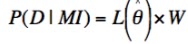
Lets express the numerator in a new form by defining the Ockham factor, W (for William, I guess), as follows:

(6)

which is the same as

(7)

from which it is clear that

(8)

Now we can write the ratio of the probabilities associated with the two models, M_j and M_k, in terms of expression (5):

(9)

So the orthodox estimate is multiplied by two additional factors: the prior odds ratio and the ratio of the Ockham factors. Both of these can have strong impacts on the result. The prior odds for the hypotheses under investigation can be important when we already had reason to prefer one model to the other. In parameter estimation, we’ll often see that these priors make negligible difference in cases where the data carry a lot of information. In model comparison, however, prior information of another kind can have enormous impact, even when the data are extremely informative. This is introduced by the means of the Ockham factor, which can easily overrule both the prior odds and the maximum-likelihood ratio.

In light of this insight, we should take a moment to examine what the Ockham factor represents. We can do this in the limit that the data are much more informative than the priors, and the likelihood function is sharply peaked at  (which is quite normal, especially for a well designed experiment). In this case, we can estimate the sharply peaked function L(θ) as a rectangular hyper-volume with a ‘hyper-base’ of volume V, and height . We choose the size of V such that the total enclosed likelihood is the same as the original function:

(10)

We can visualize this in one dimension, by approximating the sharply peaked function below by the adjacent square pulse, with the same area:

Since the prior probability density P(θ | MI) varies slowly over the region of maximum likelihood, we observe that

(11)

which indicates that the Ockham factor is a measure of the amount of prior probability for θ that is packed into the high-likelihood region centered on , which has been singled out by the data. We can now make more concrete how this amount of prior probability in the high likelihood region relates to the ‘simplicity’ of a model by noting again the consequences of augmenting a model with an additional free parameter. This additional parameter adds another dimension to the parameter space, which, by virtue of the fact that the total probability density must be normalized to unity, necessitates a reduction of magnitude of the peak of P(θ | MI), compared to the low-dimensional model. Lets assume that the more complex model is the same as the simple one, but with some additional terms patched in (the parameter sample space for the smaller model is embedded in that of the larger model).  Then we see that it is only if the maximum-likelihood region for the more complex model is far from that of the simpler model, that the Ockham factor has a chance to favor the more complex model.

For me, model comparison is closest to the heart of science. Ultimately, a scientist does not care much about the magnitude of some measurement error, or trivia such as the precise amount of time it takes the Earth to orbit the sun. The scientist is really much more interested in the nature of the cause and effect relationships that shape reality. Many scientists are motivated by desire to understand why nature looks the way it does, and why, for example, the universe supports the existence of beings capable of pondering such things. Model comparison lifts statistical inference beyond the dry realm of parameter estimation, to a wonderful place where we can ask: what is going on here? A formal understanding of model comparison (and a resulting intuitive appreciation) should, in my view, be something in the toolbox of every scientist, yet it is something that I have stumbled upon, much to my delight, almost by chance.   

Ockham's Razor

Numquam ponenda est pluralitas sine necessitate.

- attributed to William of Ockham, circa 1300.

Translation: “Plurality should not be posited without need.”

The above quotation is understood to be a heuristic principle to aid in the comparison of different explanations for a set of known facts.

The principle is often restated as:

          ‘The simplest possible explanation is usually the correct explanation.’

This idea is frequently invoked by scientists, engineers, or any other class of person involved in rational decision making, very often without thinking. We know instinctively, for example, that when trying to identify the cause of the force between two parallel current-carrying wires, it is useless to contemplate the presence of monkeys on the moon. But this is the most trivial form of application of the Ockham principle, specifying our preferred attitude to entities of no conceivable relevance to the subject of study.

Less trivial applications occur when we contemplate things that would have an effect on the processes we study. In such cases it is still widely and instinctively accepted that we should postulate only sufficient causal agents to explain the recorded phenomena. We tend to see the ‘simplicity’ of an explanation, therefore, to be advantageous. Mathematically, this is related to the complexity of the mathematical model with which we formulate our description of a process.  A linear response model, for example, when it gives a good fit, is seen as more desirable than a quadratic model. This may be partly related to the greater ease with which a linear model can be investigated mathematically, but there is also a feeling that if the fit is good, then the linear model probably is the true model, even though the quadratic model will always give a better fit (lower minimized residuals) to noisy data.

Two problems arise if we try to make the Ockham principle objective:

(i)               How do we define the ‘simplicity’ of a model?

(ii)              How are we to determine when it is acceptable to reject a model in

                   favor of one less simple?  

A slightly loose definition of the simplicity of a model is the ease with which it can be falsified. That is, if a model makes very precise predictions, then it is potentially quickly disproved by data, and is considered simple. With a Bernoulli urn, for example, known to contain balls restricted to only 2 possible colours, the theory that all balls are the same colour is instantly crushed, if we draw 2 balls of different hues. An alternate model, however, that the urn contains an equal mixture of balls of both colours is consistent with a wider set of outcomes – if we draw 10 balls, all of the same colour, then it is less likely, but still possible that that there are balls of both colour in the urn.

To make the definition of simplicity more exact, we can say that the simpler model has a less dispersed sampling distribution for the possible data sets we might get if that model is true. P(D | M, I) is more sharply concentrated.

Mathematical models of varying numbers of degrees of freedom can also succumb to a characterization of their relative simplicity using this definition. If one finds that a simple model does not exactly fit the data, then one can usually quite easily ‘correct’ the model by adding some new free parameter, or ‘fudge factor.’ Adding an additional parameter gives the model a greater opportunity to reduce any discrepancies between theory and data, because the sampling distribution for the data is broader – the additional degree of freedom means that a greater set of conceivable observations are consistent with the model, and P(D | M, I) is spread out more thinly. This, however, means that it is harder to falsify the model, and it is this fact that we need to translate into some kind of penalty when we calculate the appropriateness of the model.

To see how we can use Bayes’ theorem to provide an objective Ockham’s razor, I’ll use a beautiful example given by Jeffreys and Berger¹, in ‘Sharpening Ockham’s Razor on a Bayesian Strop.’ The example concerns the comparison of competing theories of gravity in the 1920s: Einstein’s relativity, which we denote by proposition E, and a fudged Newtonian theory, N, in which the inverse-square dependence on distance is allowed instead to become d^-(2+ε), where ε is some small fudge factor. This was a genuine controversy at that time, with some respected theorists refusing to accept relativity. 

The evidence we wish to use to judge these models is the observed anomalous motion of the orbit of Mercury, seen to differ from ordinary Newtonian mechanics by an amount, a = 41.6 ± 2.0 seconds of arc per century. The value, α, calculated for this deviation using E was 42.9’’, a very satisfying result, but we will use our objective methodology to ascertain whether in light of this evidence, E is more probably the truth than N, the fudged Newtonian model. In order to do this we need sampling distributions for the observed discrepancy, a, for each of the models.

For E, this is straightforward (assuming the experimental error magnitude is normally distributed):

For N, the probability to observe any particular value, a, depends not only on the experimental uncertainty, σ, but also on the sampling distribution for α, the predicted value for the anomalous motion. This is because α is not fixed, due to the free parameter, ε. We can treat α as a nuisance parameter for this model:

To find P(α | N), we note that a priori, there is no strong reason for the discrepant motion to be in any given direction, so positive values are as likely as negative ones. Also large values are unlikely, otherwise they would be manifested in other phenomena. From studies of other planets, a value for α > 100’’ can be ruled out. Therefore, we employ another Gaussian distribution, centered at zero and with standard deviation, τ, equal to 50’’.

P(a | N) can then be seen to be a Gaussian determined by the convolution of the measurement uncertainty and the distribution for α:

We’ll consider ourselves to be otherwise completely ignorant about which theory should be favored, and assign equal prior probabilities of 0.5.

Bayes’ theorem in this case is:

and so we get the posterior probabilities: P(E | a, I) = 0.966 and P(N | a, I) =  0.034, which is nearly 30 times smaller. Because the fudged Newtonian theory has 2 uncertainties, the measurement error, and the free parameter, ε, the sampling distribution for the possible observed discrepancy, a, is spread over a much broader range.

Plotting the sampling distributions for the observed value, a, for each of the two models reveals exactly why their posterior probabilities are so different:

Because E packs so much probability into the region close to the observed anomaly, it comes out far more highly favored than N. If the actual observation was far from 40’’, then the additional degree of freedom of model N would be seen to be vindicated.

We can perform a sensitivity analysis to see whether we would have had a radically different result upon choosing a slightly different value for τ. Plotted below are the results for the same probability calculation just performed, but with a large range of possible values of τ:

The result shows clearly that we are not doing a great disservice to the data by arbitrarily setting τ at 50’’. The total absolute variation of P(E | a, I) is less than 0.04. We can also experiment with the prior probabilities, but remarkably, the posterior probability for the Einstein theory, P(E | a, I) falls only to 0.76 if P(E | I) is reduced to 0.1. This illustrates the important point that as long as our priors are somehow reasonably justified, the outcome is very often not badly affected by the slight arbitrariness with which they are sometimes defined.

Note that in order for the posterior probability, P(E | a, I), to be lowered to 0.5, the same value as the prior, we would need to increase the experimental uncertainty, σ, to more than 1000’’. This gives some kind of measure of the large penalty paid by introducing one extra free parameter.

The Ockham principle is a vague rule of thumb that, as we've just seen, can be derived from a much more general and quantitative principle, namely Bayes’ theorem. The fact that many people have been intuitively able to appreciate the validity of Ockham’s razor for roughly seven centuries is suggestive of how close Bayes’ theorem is to the way that human brains perform plausible reasoning. And why should it be any different? Bayes’ theorem is derived from robust logical principles, and it is no surprise that natural selection might favor information processing algorithms that mimic those principles.

In its original informal statement, Ockham’s razor may let us down in some cases, where there is strong prior information, where the ‘simplicity’ of two models is difficult to compare using our ill-defined, intuitive understanding of the term, or where the balance between goodness of fit and the penalty for complexity is too close for intuition alone to judge. The more general application of plausible reasoning using Bayes’ theorem, however, provides the best possible quality of inference, allows all these hard-to-define qualities (prior belief, simplicity, goodness of fit) to be objectively quantified, and puts model comparison on a firm logical basis.

---

[1] W.H. Jeffreys and J.O. Berger, ‘Sharpening Ockham’s Razor on a Bayesian Strop,’ Purdue University technical report #91-44C, August 1991 (Download here.)